AFLR3 Example Cases Tutorial
Data files for several AFLR3 sample cases are provided. Package archives
with all of the example cases are provided in aflr3-examples.tar.gz
(tar-gzip archive for Linux/MacOSX) and aflr3-examples.zip (zip archive for Windows).
Copy the package archive files and unpackage them in a location of your
choosing to run the example cases. All cases have relatively coarse spacing and
require minimal resources. The input surface mesh files provided for the sample
cases are ASCII formatted SURF type files, with one NASTRAN type exception. In
the following case examples the output mesh file is a big-endian double
precision C-binary (.b8) UGRID type file. Alternative file types can be used.
An isotropic element volume mesh can be generated for any of the sample cases
using the following. By default the output volume mesh with be a binary format
UGRID file type named case_name.b8.ugrid.
aflr3 -i case_name
For example, to generate an isotropic mesh inside a cube enter the following.
aflr3 -i cube
Note that the case name can include a trailing dot (for Linux/MacOSX tcsh, etc.
users that use the tab key). The trailing dot is ignored.
aflr3 -i cube.
When the case name only is specified AFLR3 will search for a file with
that case name and a file type appropriate for an input mesh. Surface mesh only
file types are searched for before considering ones that could be either a
surface or volume mesh. The full file name can also be specified.
aflr3 -i cube.surf
See the AFLR3 documentation
for information on available options and usage. Alternatively you can view
text-based documentation at the command line with the following command.
aflr3 -help
A number of systems can be used to visualize the resulting volume mesh.
Use of a visualization systems may require conversion of the output mesh
file to one of another type (Ensight, FieldView, Mesh, and others are available).
AFLR3 can be used to convert the file using the following
command.
aflr3 -convert -i case_name.b8.ugrid -o
case_name.output_type
Alternatively, the UG_IO file converter UGC can be used with the
following command.
ugc case_name.b8.ugrid case_name.output_type
See the UGC documentation for a
description of usage and options. Alternatively you can view text-based
documentation at the command line with the following command.
ugc -help
Note that AFLR3 can output the mesh file in another file type just after
generation. However, subsequent conversion to another file type may not be
possible if the original output mesh is not a UGRID file type. The
documentation describes whether or not a file type can be used as an input mesh
for conversion.
Several example cases are provided. TAGS files are included for most cases. The
TAGS file can be used to name components and set grid related parameters for
each unique surface ID. A TAGS file is not required to use AFLR3.
However, it can be useful to set grid boundary conditions and parameters.
SolidMesh generates a TAGS file automatically. SolidMesh can also be
used to set the information and create a TAGS file for cases with input surface
meshes that are generated in another system. Alternatively the TAGS file can be
created in a text editor.
Isotropic Mesh Generation
No options are typically required for most isotropic tetrahedral mesh
cases. Additional options are usually only required for applications with
specific sizing needs or specifying grid BCs for embedded/transparent
surfaces.Example cases for isotropic type mesh generation are listed below
along with appropriate options.
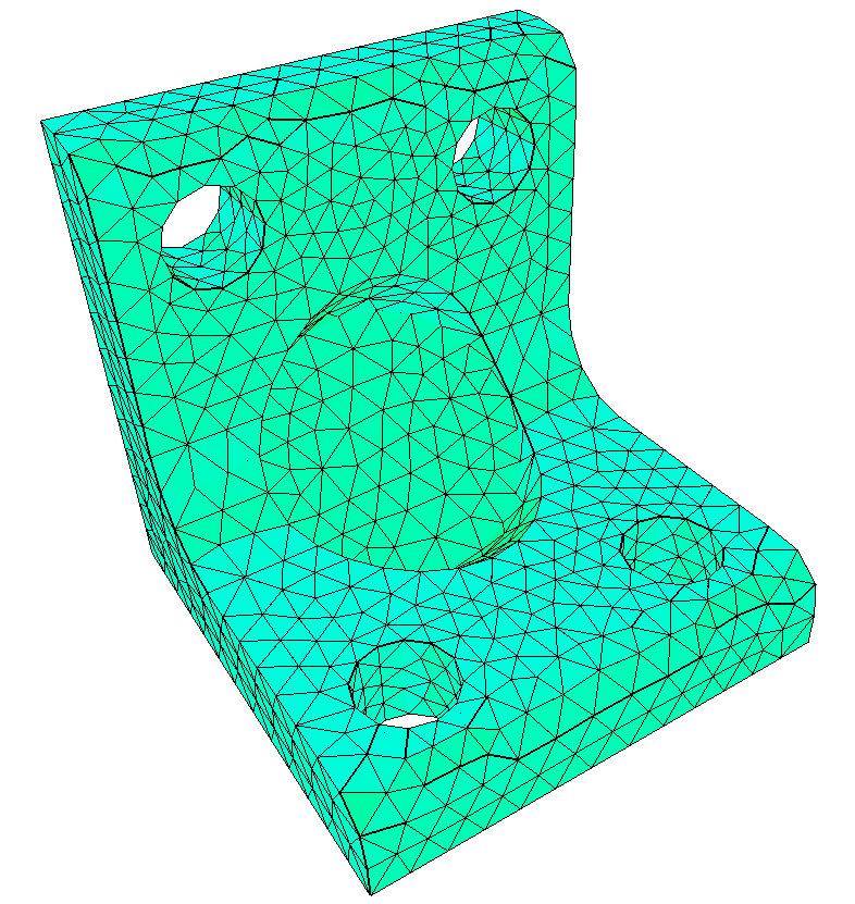
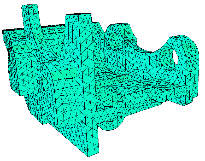
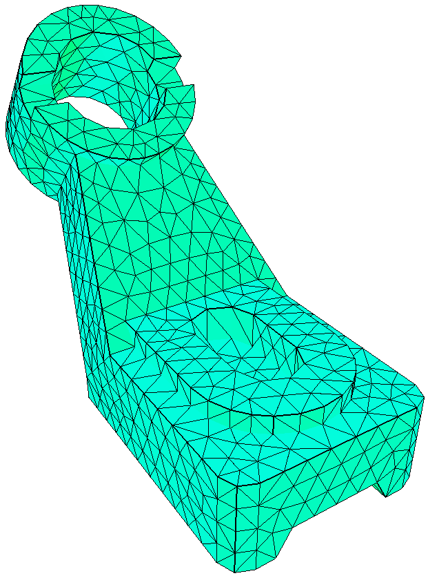
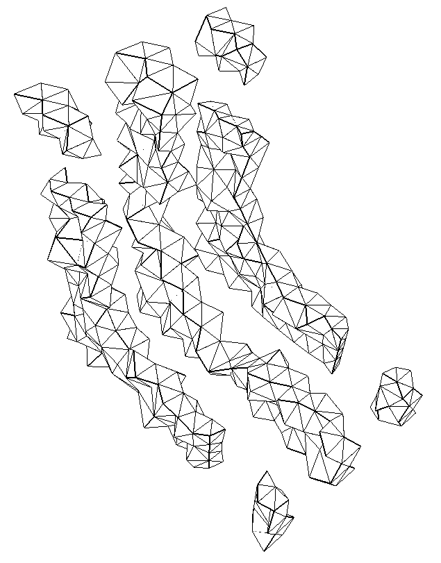
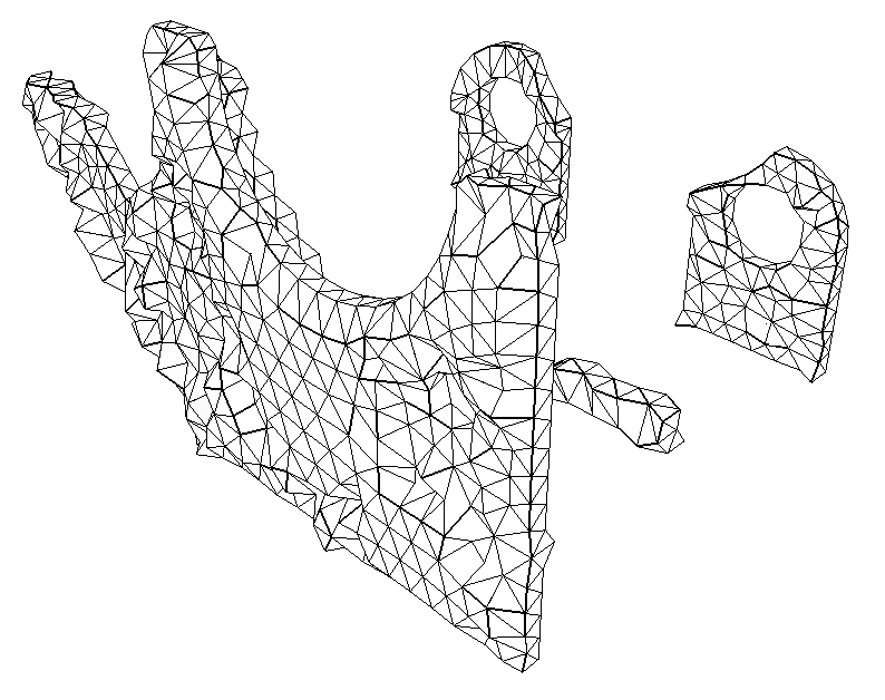
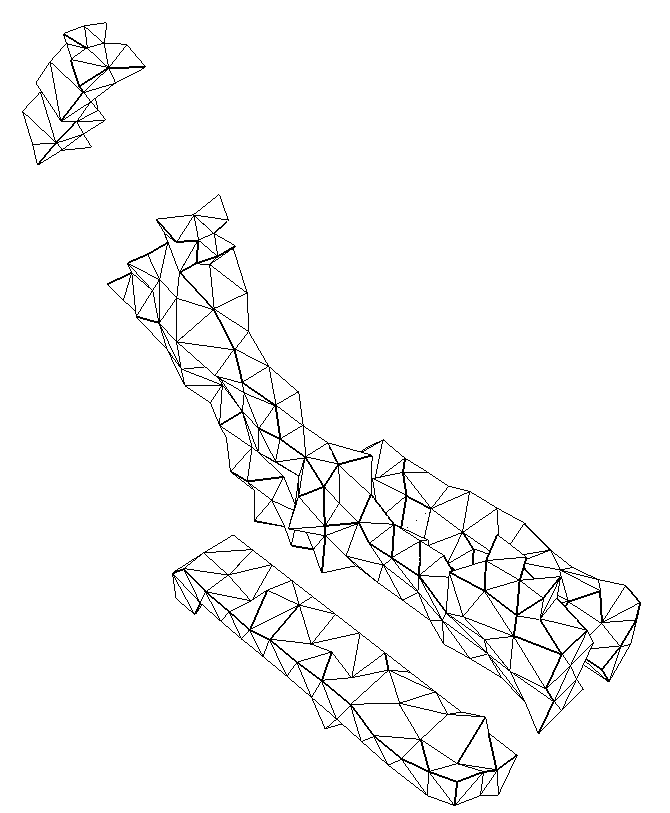
Mechanical parts. The bracket2, bracket4, cami, and cover_plate cases
are mechanical parts with surface meshes suitable only for an isotropic type
volume mesh.
aflr3 -i bracket2
aflr3 -i bracket4
aflr3 -i cami
aflr3 -i cover_plate
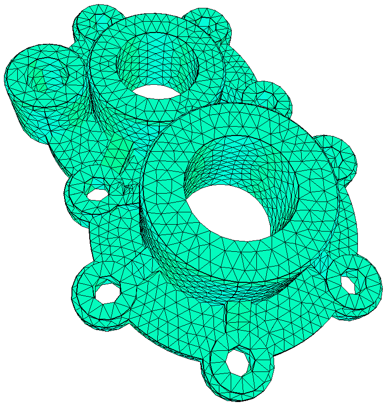
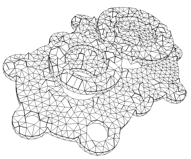
Mechanical parts with quad faces. The plug and plug2 cases are
mechanical parts with surface meshes that contain predominantly quad faces and
are suitable for an isotropic type volume mesh. The plug2 case is the same as
the plug case with a finer mesh. The quad faces can be preserved as quads with
pyramid transition using the mquadp=1 option.
aflr3 -i plug mquadp=1
aflr3 -i plug2 mquadp=1
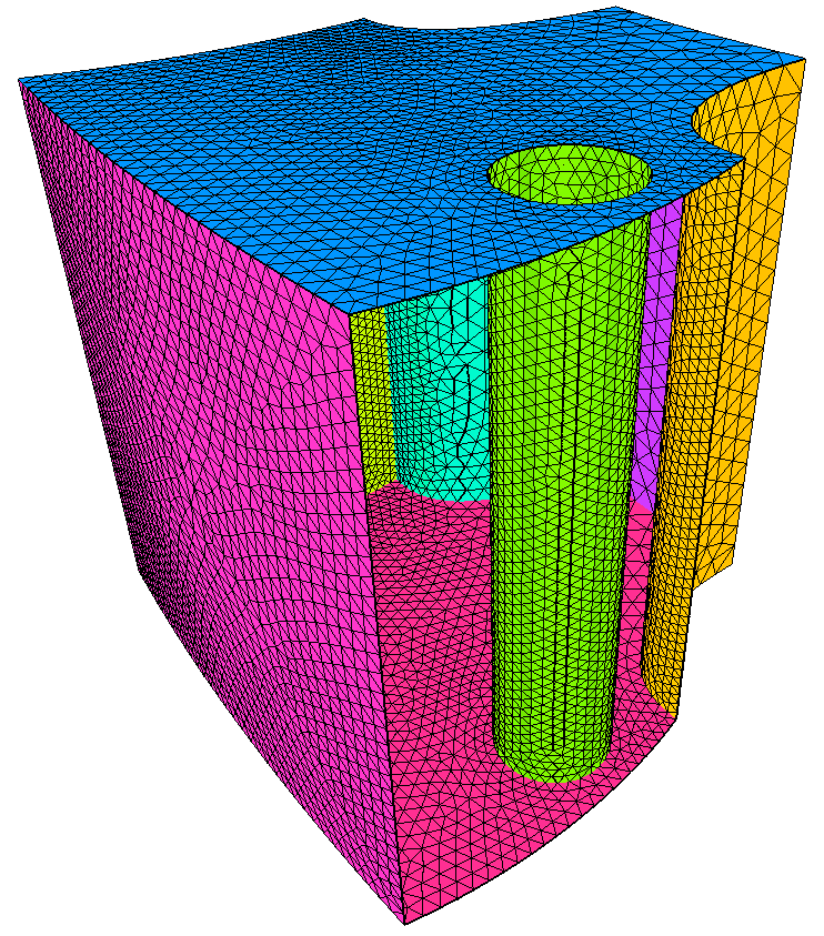
Multi-material assembly. The em case is a case suitable for
an isotropic mesh. Appropriate grid boundary conditions are set within the
surface grid file and the mesh can be generated with the following.
aflr3 -i em
If the input surface mesh does not contain grid boundary conditions then they
can be completely specified on the command line using option flags as shown
below. A TAGS file could also be used to set this information. See
documentation for more information on grid boundary condition values. Here a
Grid_BC value of 1 denotes a standard solid surface and a value of 5 denotes an
embedded or transparent surface that has volume mesh on both sides. For this
case the inner solid objects are ID=2, ID=8, and ID=14; the transparent objects
are ID=3, ID=4, ID=5, ID=6, and ID=9; and the outer solid object is ID=7.
aflr3 -i em -BC_IDs 2,3,4,5,6,7,8,9,14 -Grid_BC_Flag
1,5,5,5,5,1,1,5,1
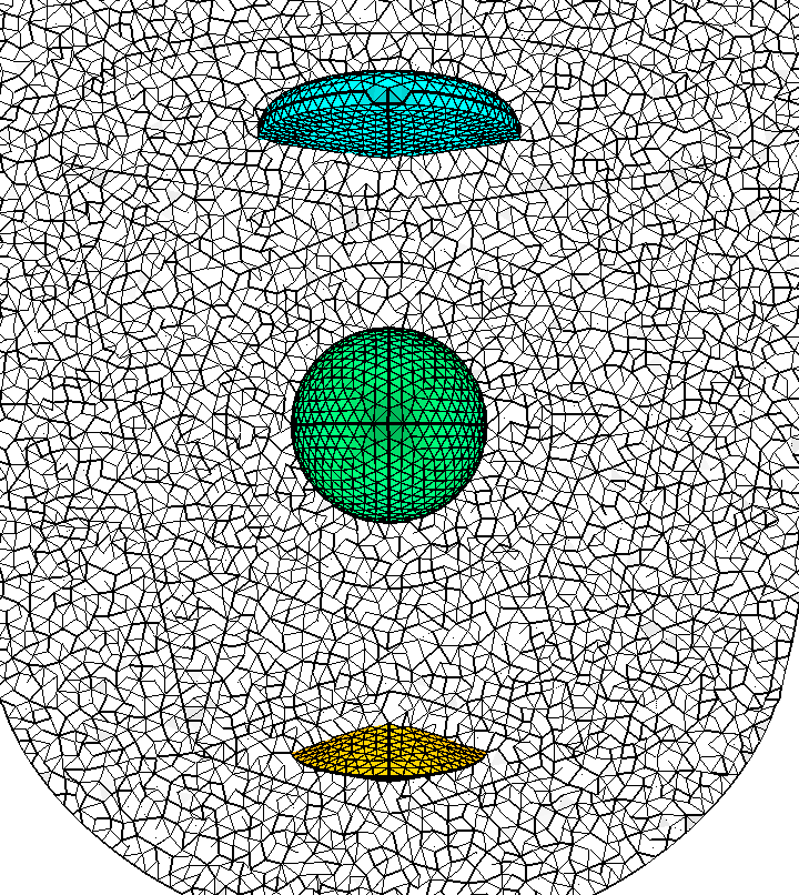
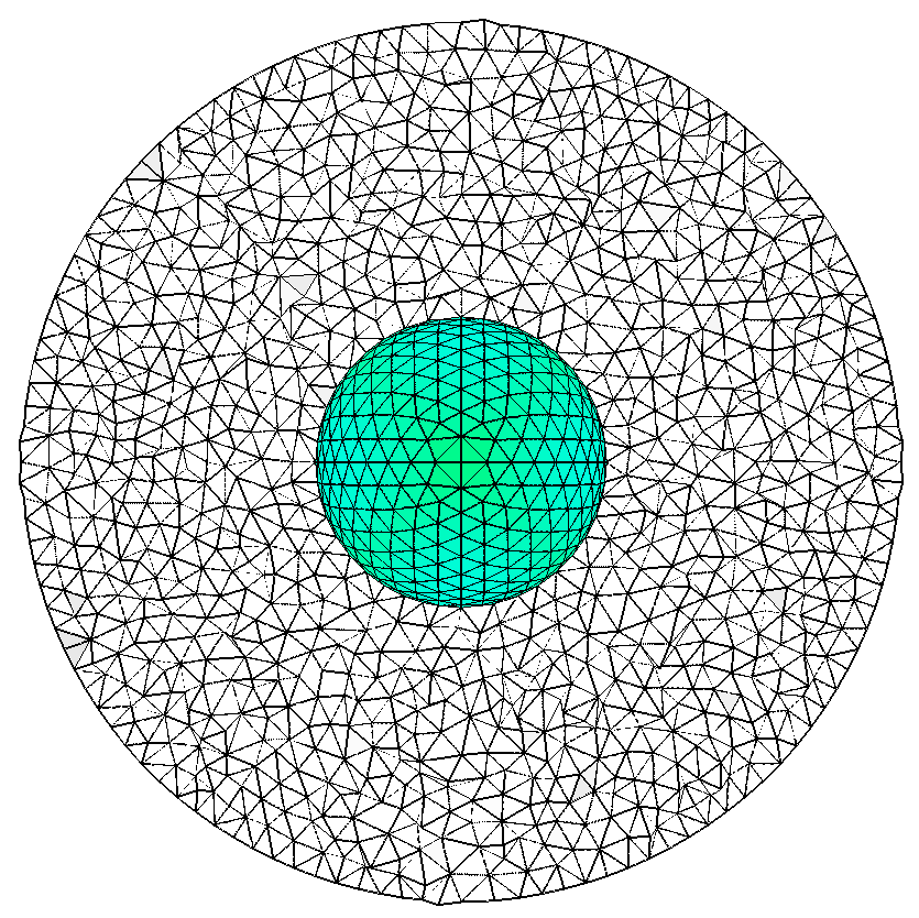
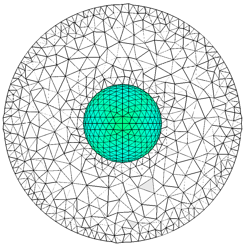
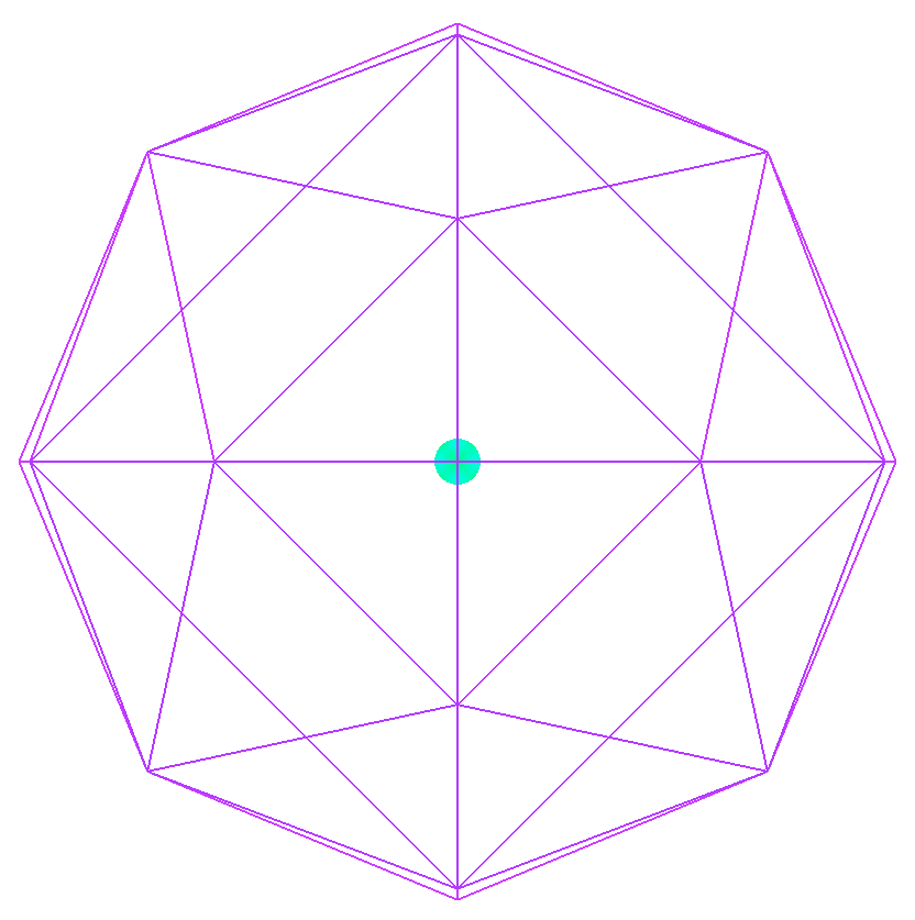
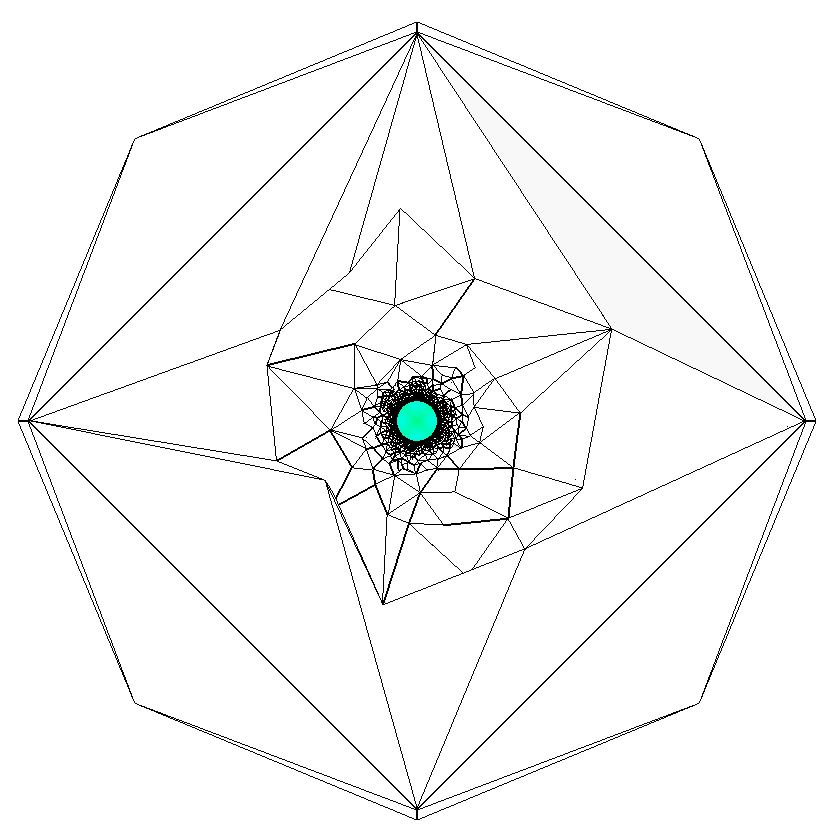
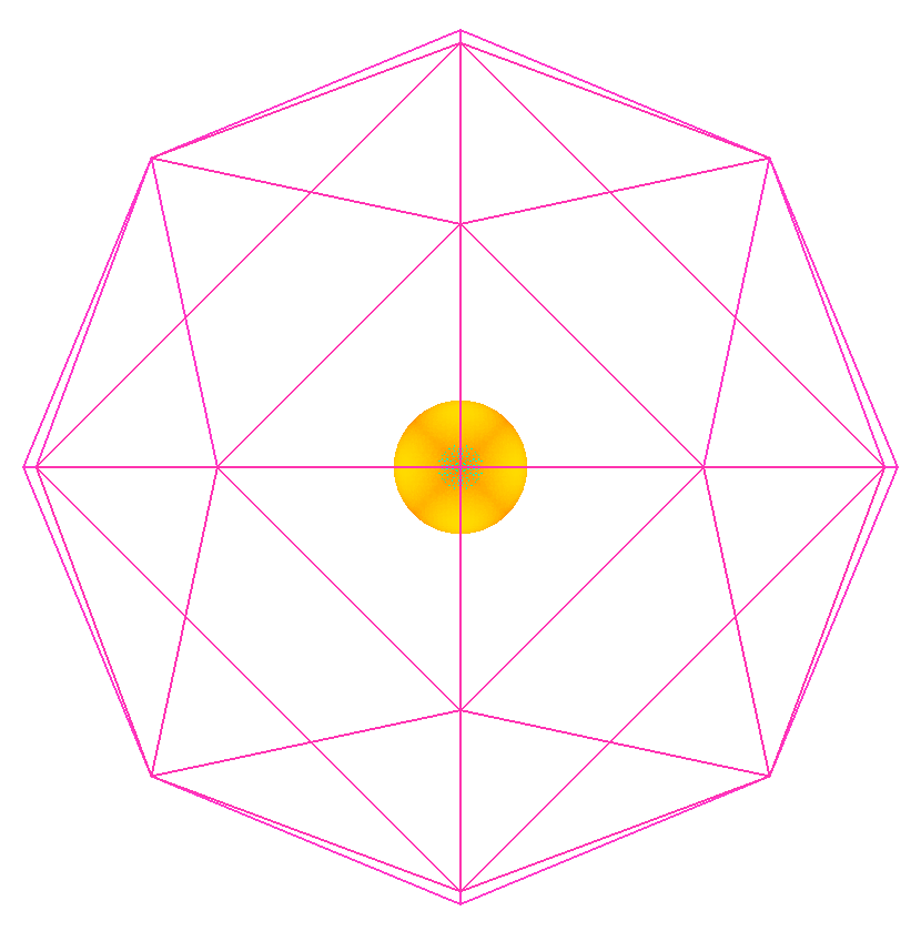
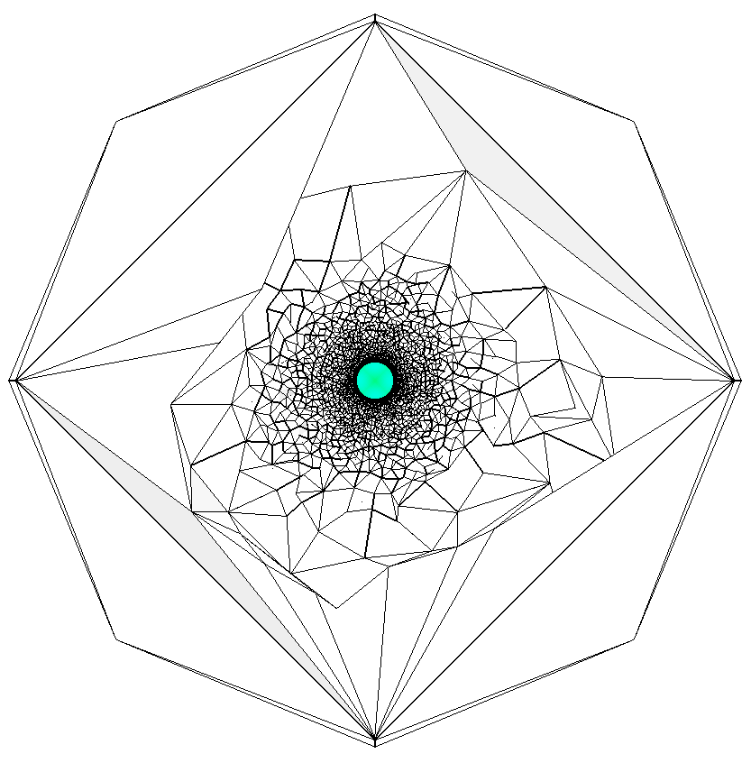
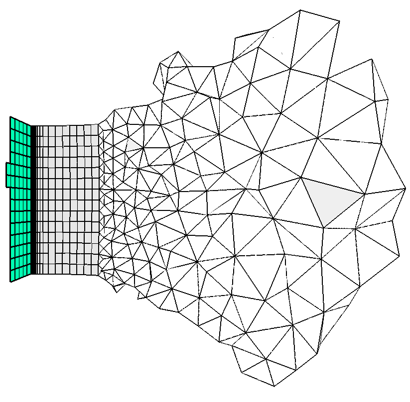
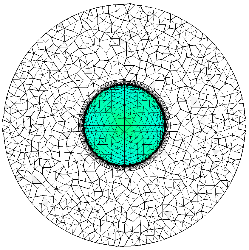
Control of isotropic field spacing. A simple case of a sphere of radius
1 inside of a sphere of radius 3 is useful to demonstrate control of isotropic
field spacing. By default spacing is determined by interpolation between
boundaries and the field elements have a slightly larger node spacing than the
boundary surfaces (controlled by cdf).
aflr3 -i spheres_1_3
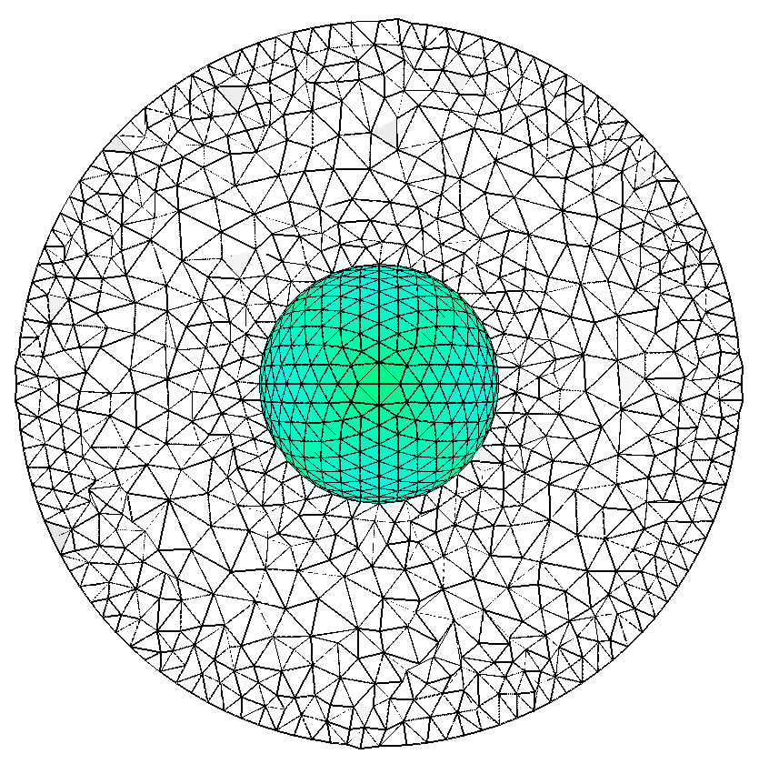
In some applications (EM analysis) it may be advantageous to limit the maximum
spacing even when overall spacing is relatively uniform. Adding the -dfmax
option adds additional grid generation passes to continue point creation until
the maximum spacing is less than or equal to the value specified. This may not
be possible if any of the surface faces have large spacing. And, if the surface
spacing varies much then it will further reduce element quality in regions
where the surface spacing is larger.
aflr3 -i spheres_1_3 -dfmax 0.16
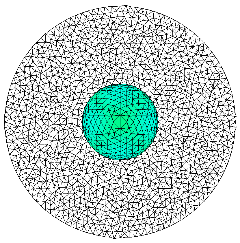
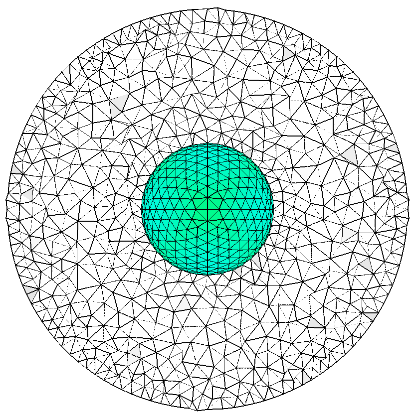
In other cases it may be desired to increase the element size away from the
boundary surfaces. Adding the option -grow, -grow1, -grow2 or -grow3 will
change the default interpolation of spacing to a growth based method. Moderate
growth is provided with the option -grow2. Use of growth usually always
degrades quality, whether the boundary spacing is uniform or varied.
aflr3 -i spheres_1_3 -grow1
The -grow1 option uses a default exclusion zone factor of 1 element (cdfs=1).
Within the exclusion zone the element size remains relatively constant. Slight
growth is allowed and not a hard limit. Using the option cdfs=4 along with
-grow1 will use the increase the allowable exclusion zone factor.
aflr3 -i spheres_1_3 -grow1 cdfs=4
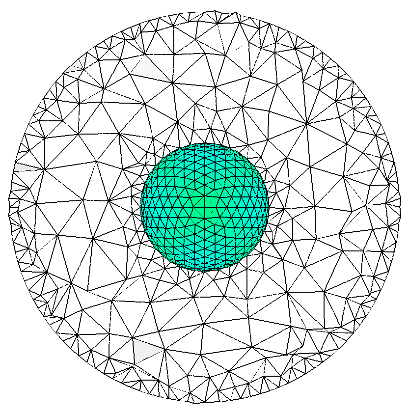
The -grow1 option uses a geometric growth rate of 1.2. The default value for
growth (also used to limit growth in element size due to variation in spacing)
is 1.1. Simply turning on geometric growth spacing evaluation with the option
mdf=2 will use the default value for growth. This is equivalent to using the
option -grow 1.1.
aflr3 -i spheres_1_3 mdf=2
And, of course growth can be increased further, at the expense of element shape
quality. Using the option -grow2 uses a higher growth rate of 1.5 and a smaller
exclusion zone factor of 0.5.
aflr3 -i spheres_1_3 -grow2
BL Mesh Generation
Additional options are required to generate a pseudo-structured
anisotropic BL type mesh adjacent to selected boundaries. Not all of the
sample cases provided are suitable for BL mesh generation. Several options are
available to control the BL mesh generation a thorough review of the
documentation is recommended. BL meshes with very different characteristics can
be generated with the appropriate options. A unique set of characteristics that
is suitable for particular applications and solvers can be obtained. It is
recommended to develop the appropriate set of options that meets the needs of
your cases with a relatively simple configuration. Example cases for BL type mesh
generation are listed below along with appropriate options.
Note that AFLR3 does not generate any quality statistics after
generation of cases with a BL or SNS region. When AFLR3 generates a BL
mesh an out-of-core memory (temporary files) system is used to minimize memory
requirements and at no time is the complete mesh in memory. Consequently a post
mesh generation run must be made to generate grid quality statistics. For large
cases this can require considerable memory, as the complete mesh must be loaded
in memory. To generate grid quality statistics for an existing volume
mesh the following command can be used.
aflr3 -qstat -i case_name.b8.ugrid
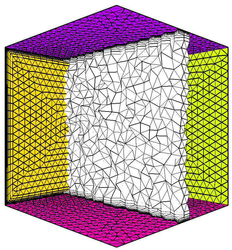
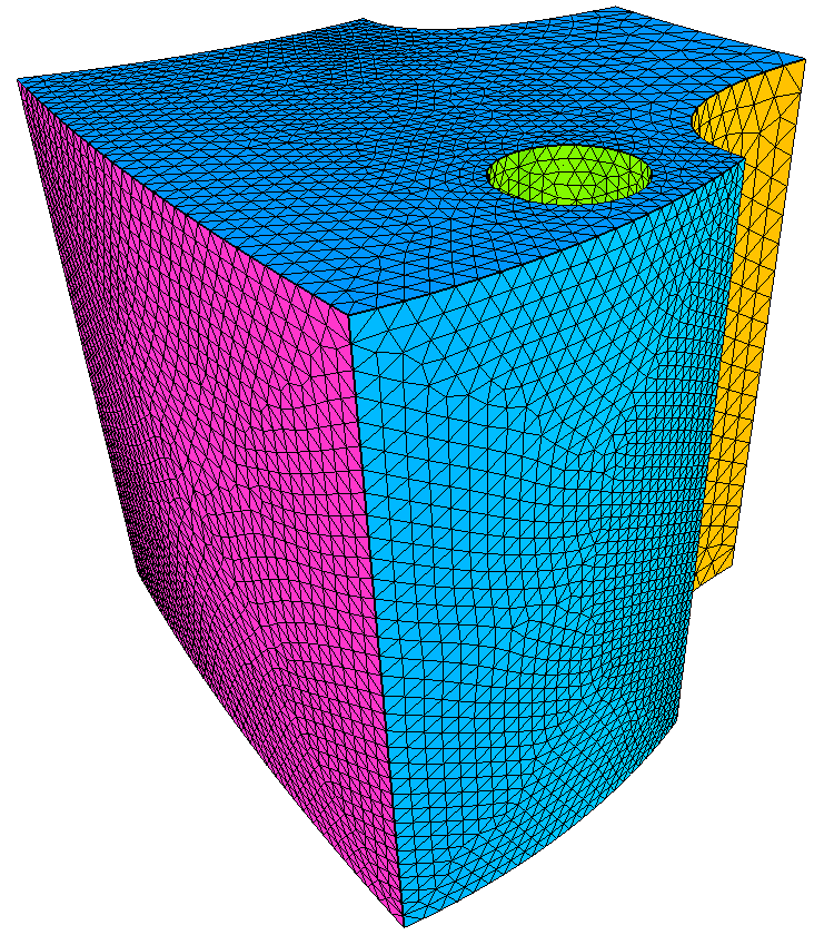
Cube with symmetry type planes. Symmetry planes are treated as surfaces
that intersect the BL region and are rebuilt within AFLR3. Note that
appropriate grid boundary conditions are set within the surface grid file.
aflr3 -i cube -blc -blds 0.00003
If the input surface mesh does not contain grid boundary conditions then they
can be completely specified on the command line using option flags as shown
below. A TAGS file could also be used to set this information. See
documentation for more information on grid boundary condition values. Here a
Grid_BC value of -1 denotes a BL generating solid surface and a value of 2
denotes a surface that intersects the BL region and that is rebuilt by AFLR3.
For this case the front and back rebuild surfaces are ID=1 and ID=2; and the BL
generating surfaces are ID=3, ID=4, ID=5, and ID=6.
aflr3 -i cube -blc -blds 0.00003 -BC_IDs 1,2,3,4,5,6
-Grid_BC_Flag 2,2,-1,-1,-1,-1
Alternatively the exact same information can be set using the -bls and -ints
options.
aflr3 -i cube -blc -blds 0.00003 -bls 1,2 -ints 3,4,5,6
A BL like region with fully specified normal spacing (SNS) can also be
generated. In this case the normal spacing is specified differently on the left
and right surfaces and all other surfaces are treated as ones that intersect
the BL/SNS region and are rebuilt within AFLR3. The transition to the
isotropic region continues from the specified layers at a constant growth rate
(see -snsr option). See the documentation for more information on options
related to SNS mode.
aflr3 -i cube -snsc -snsids 5,6 -ints 1,2,3,4 -snsi 1,5,1,6
\
-snss 0.0,0.1,0.2,0.3,0.4,0.5,0.0,0.2,0.4,0.6,0.8,1.0
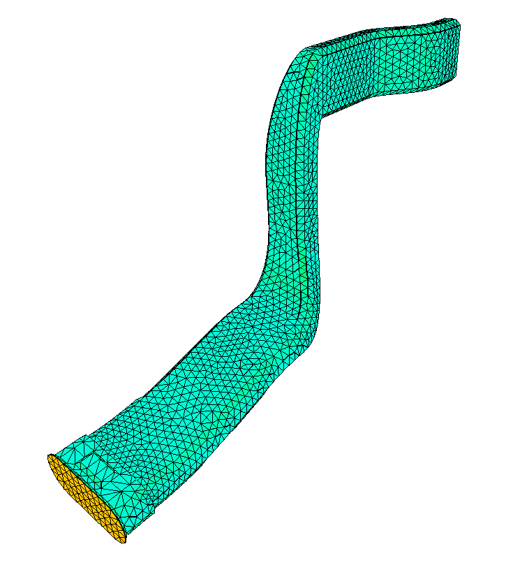
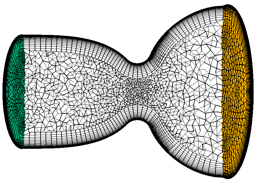
Curved duct with inlet and outlet. Inlet and outlet are treated as
surfaces that intersect the BL region and are rebuilt within AFLR3. Note
that appropriate grid boundary conditions are set within the surface grid file.
aflr3 -i curved_duct -blc -blds 0.00003
If
the input surface mesh does not contain grid boundary conditions then they can
be completely specified on the command line using option flags as shown below.
A TAGS file could also be used to set this information. For this case the inlet
and outlet rebuild surfaces are ID=2 and ID=3; and the BL generating nozzle
wall surface is ID=4. Note that the -bls option list only contains one ID and
must be terminated with a comma.
aflr3 -i curved_duct -blc -blds 0.00003 -bls 4, -ints 2,3
Defroster duct with inlet and outlet. Inlet and outlet are treated as
surfaces that intersect the BL region and are rebuilt within AFLR3. Note
that appropriate grid boundary conditions are set within the surface grid file.
aflr3 -i defroster -blc -blds 0.00003
If the input surface mesh does not contain grid boundary conditions then they
can be completely specified on the command line using option flags as shown
below. A TAGS file could also be used to set this information. For this case
the inlet and outlet rebuild surfaces are ID=1 and ID=2; and the BL generating
defroster duct wall surface is ID=3. Note that the -bls option list only
contains one ID and must be terminated with a comma.
aflr3 -i defroster -blc -blds 0.00003 -bls 3, -ints 1,2
Vent with inlet and outlet. Inlet and outlet are treated as
surfaces that intersect the BL region and are rebuilt within AFLR3. For
this case the input surface mesh is a NASTRAN type and does not contain any
grid boundary condition information. By default all surfaces in such cases are
set to BL generating surfaces. Option flags can be added to set the BCs. For
this case the inlet and outlet rebuild surfaces are ID=2 and ID=3; and the BL
generating vent wall surface is ID=1. Note that the -bls option list only
contains one ID and must be terminated with a comma.
aflr3 -i long_vent -blc -blds 0.00003 -bls 1 -ints 2,3
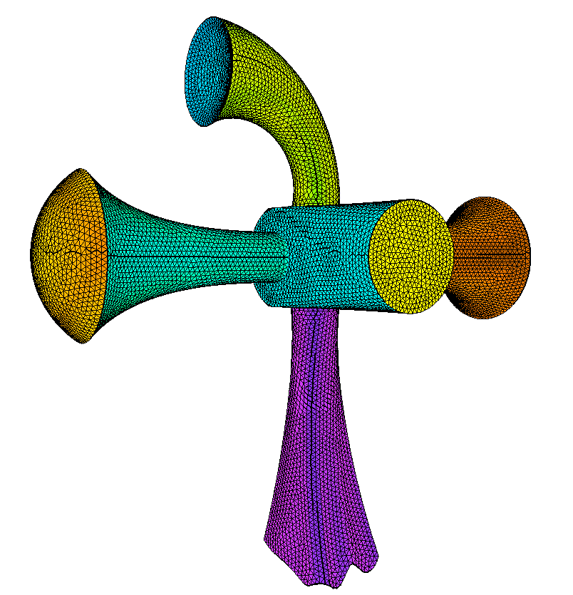
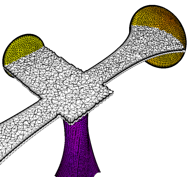
Duct with inlet and four different horn outlets. Inlet and outlets are
treated as surfaces that intersect the BL region and are rebuilt within AFLR3.
The horn outlets vary and include planar, smoothly convex, smoothly concave,
and irregularly curved outlets. The irregularly curved outlet represents an
extreme of surface curvature that while permissible, produces poor grid quality
as the BL region is constrained to follow the surface. Note that appropriate
grid boundary conditions are set within the surface grid file.
aflr3 -i horn -blc -blds 0.00003

If the input surface mesh does not contain grid boundary conditions then they
can be completely specified on the command line using option flags as shown
below. A TAGS file could also be used to set this information. Each horn and
the main body have unique IDs as do each horn outlet and the main inlet. For
this case the horn outlets and main inlet are rebuild surfaces with ID=2, ID=4,
ID=6, ID=12, and ID=13; and the BL generating horn body wall surfaces are ID=1,
ID=3, ID=5, ID=7, and ID=14.
aflr3 -i horn -blc -blds 0.00003 -bls 1,3,5,7,14 -ints
2,4,6,12,13
Rebuild surfaces that intersect the BL region. Surfaces that intersect
the BL region are rebuilt within AFLR3. They are common in BL related
applications that have inlet, outlet, and/or symmetry surfaces. In such cases
the input rebuild surfaces will be regenerated and the initial mesh replaced.
They should be sufficiently resolved to represent the surface geometry and the
interior node spacing on the surface will be driven by their bounding edge node
spacing and the actual BL region generated. AFLR3 uses a quality surface
generator, AFLR4, to regenerate rebuild surfaces. AFLR4 uses
similar algorithms combined with an automatic generation of surface uv
mapping Rebuild surfaces that are truly planar are simply generated on the
plane. Previous versions of AFLR3 used a best fit plane approximation
that required rebuild surfaces to be projectable to a plane. That restriction
sometimes required splitting of surfaces in configurations such as that
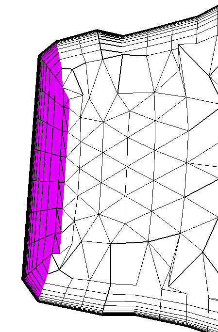
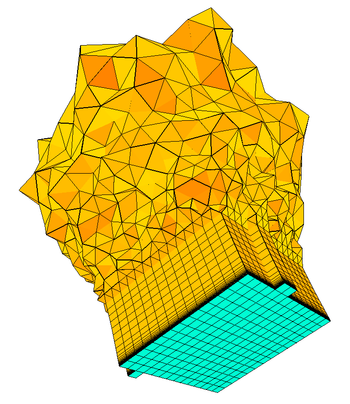
presented here. A simple case of a radial nozzle with a planar inlet rebuild
surface and curved outlet rebuild surface is useful to demonstrate the current
regeneration method. In this case the outlet is a surface of revolution and it
may be treated as one surface (as in this case) or multiple surfaces with
similar results.
aflr3 -i radial_nozzle -blc -blds 0.001
If the input surface mesh does not contain grid boundary conditions then they
can be completely specified on the command line using option flags as shown
below. A TAGS file could also be used to set this information. For this case
the inlet rebuild surface is ID=2; the radial outlet is ID=1; and the BL
generating nozzle body wall surfaces are ID=3 and ID=4.
aflr3 -i radial_nozzle -blc -blds 0.001 -bls 3,4 -ints 1,2
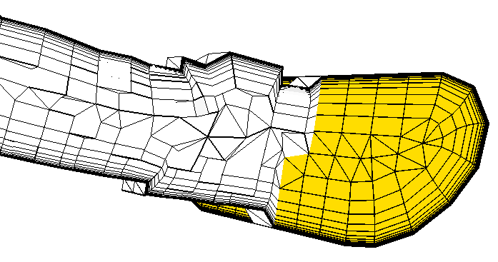
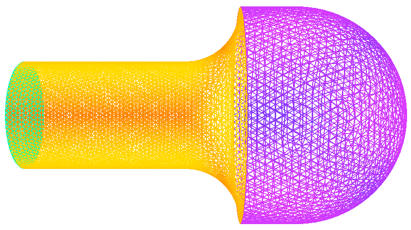
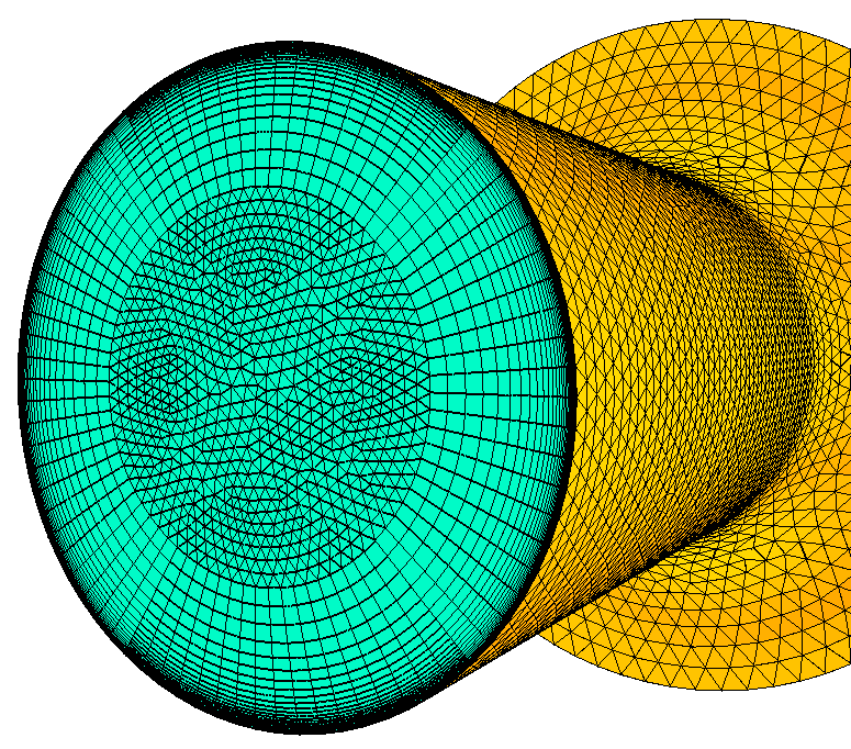
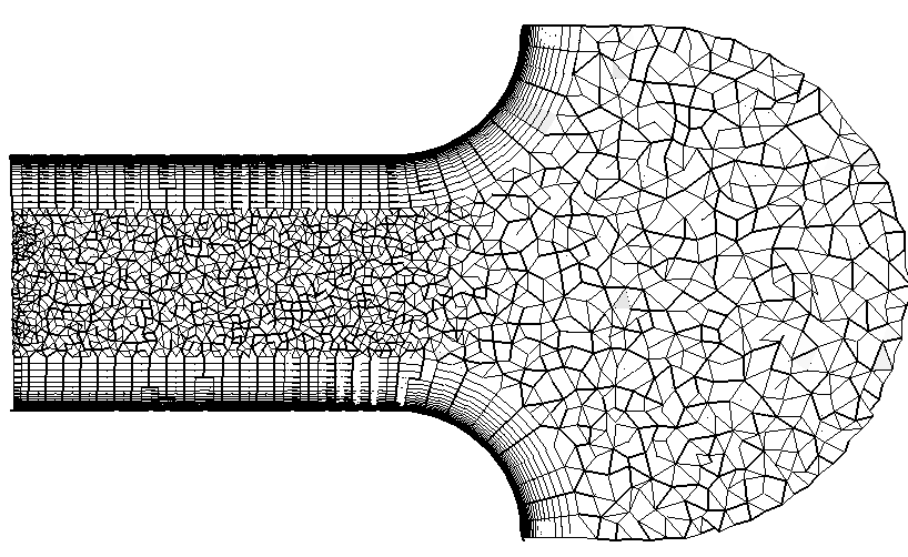
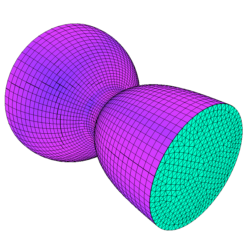
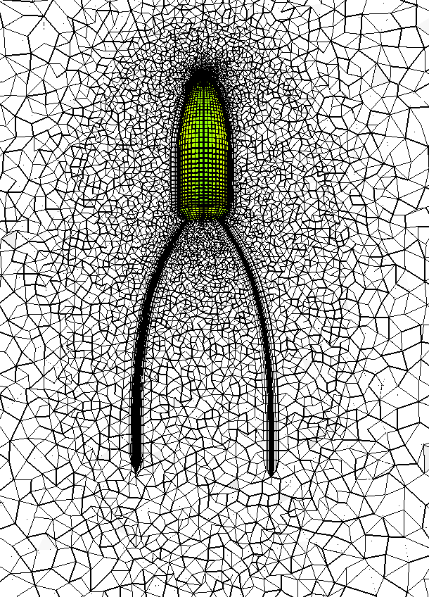
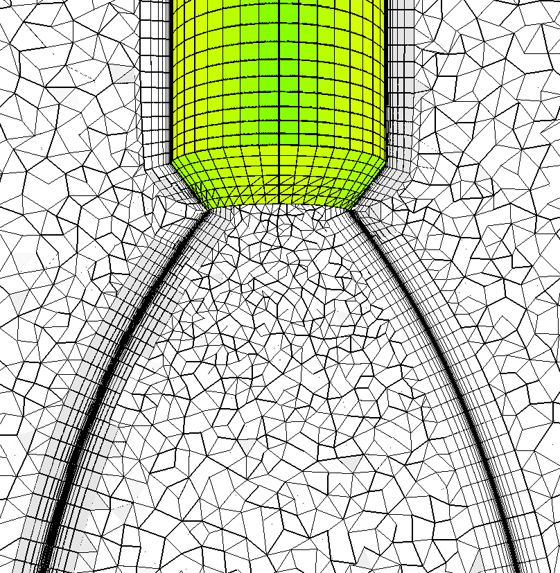
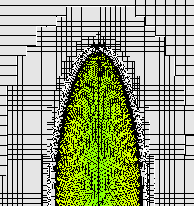
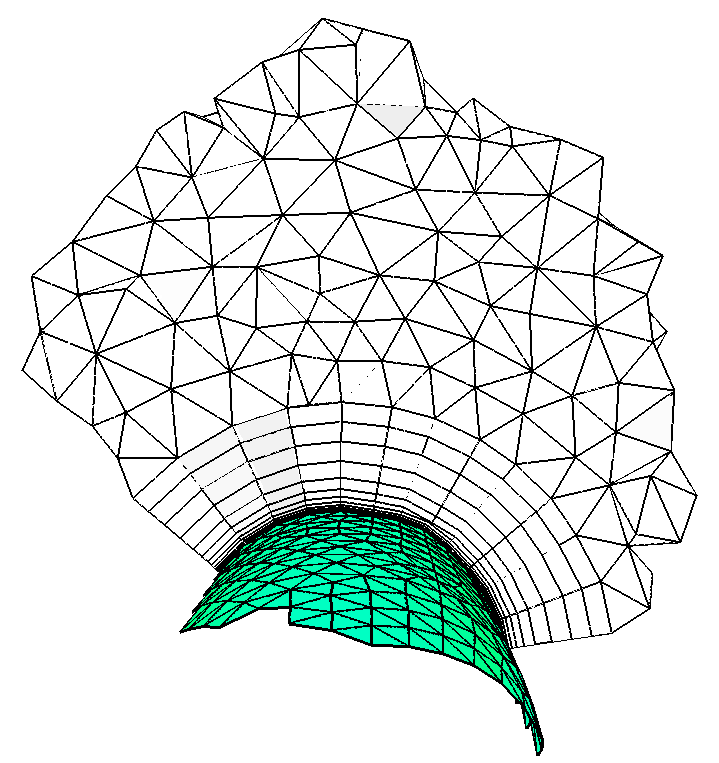
Horn with bulb exit rebuild surface that intersects the BL region. A
simple case of a cylindrical horn nozzle with a curved bulb outlet rebuild
surface to accommodate flow turning at the exit and a planar inlet rebuild
surface is also useful to demonstrate the regeneration method. In this case the
exit is a curved surface of revolution and it may be treated as one surface or
multiple surfaces with similar results.
aflr3 -i horn_bulb -blc -blrm 1.2 -blds 0.001
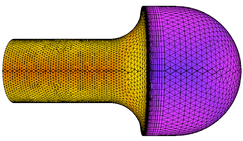
If the input surface mesh does not contain grid boundary conditions then they
can be completely specified on the command line using option flags as shown
below. A TAGS file could also be used to set this information. For this case
the bulb exit rebuild surface is ID=3; the planar inlet is ID=1; and the BL
generating cylindrical wall surface is ID=2. Note that the -bls option list only contains one ID and must
be terminated with a comma.
aflr3 -i horn_bulb -blc -blrm 1.2 -blds 0.001 -bls 2, -ints
1,3
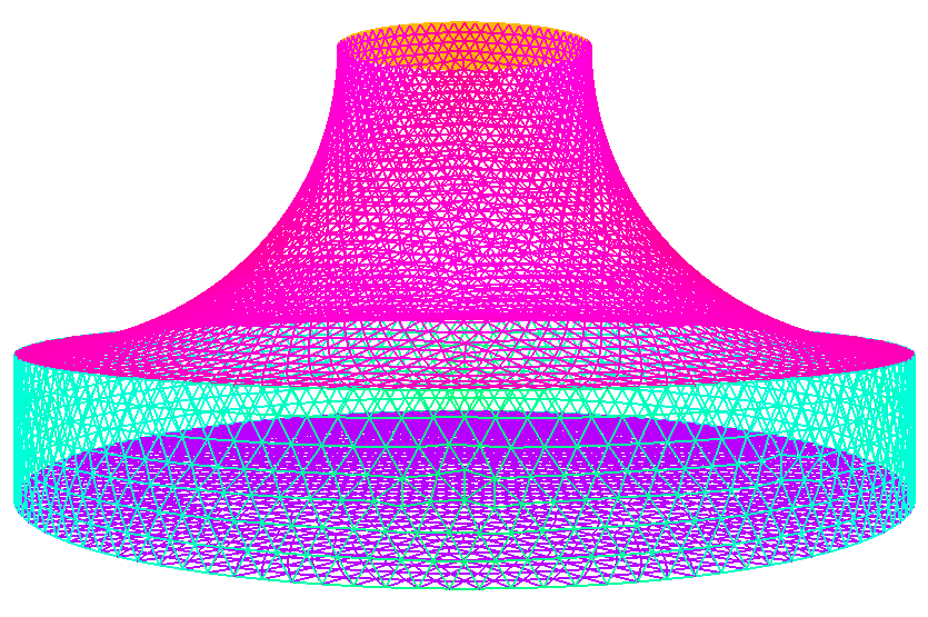
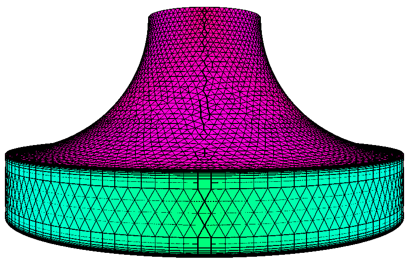
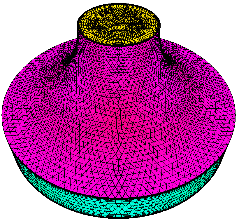
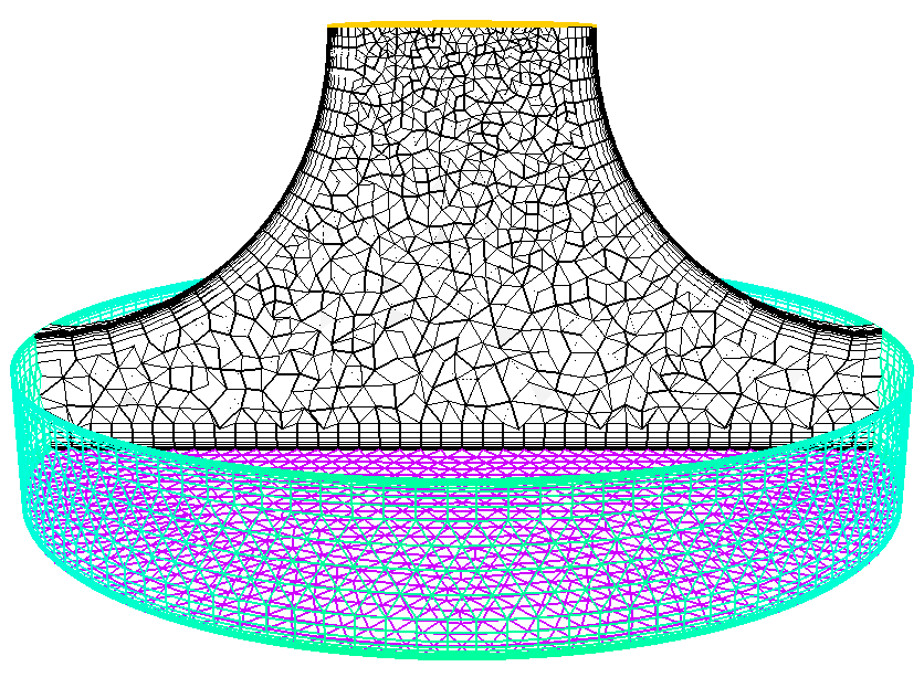
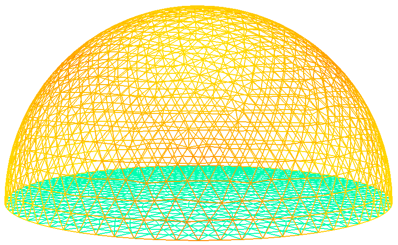
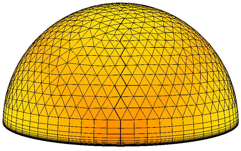
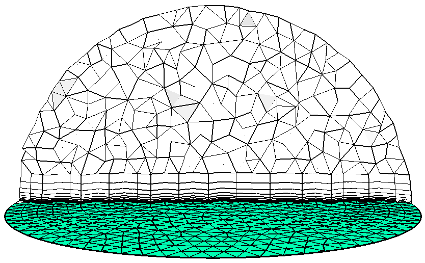
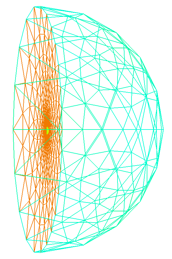
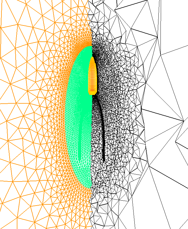
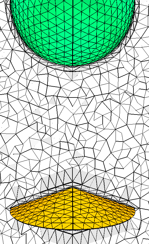
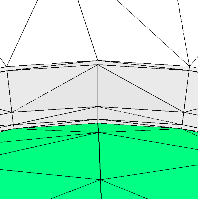
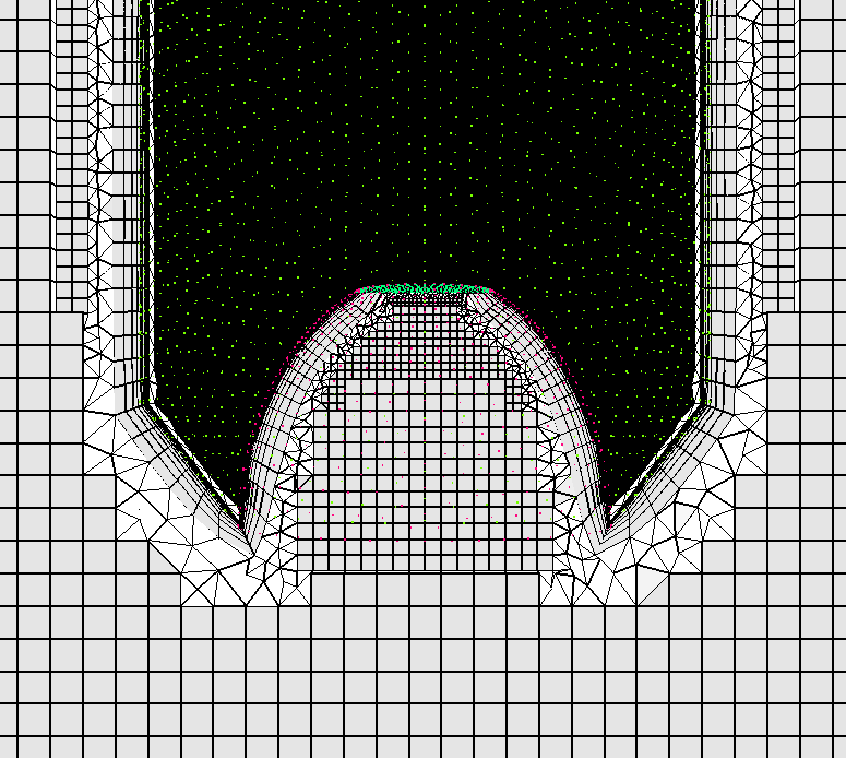
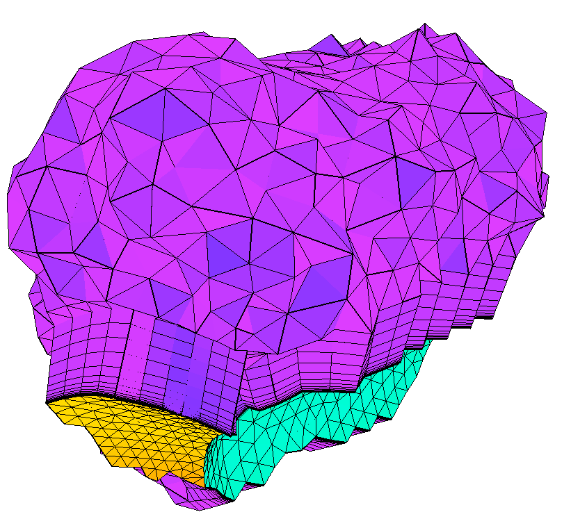
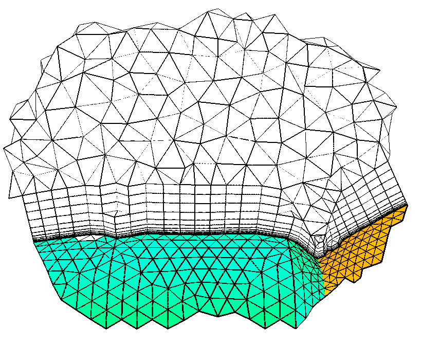
Dome rebuild surface that intersects the BL region. A simple case of a
rebuild surface that intersects the BL region on a ground plane and a planar
outlet rebuild surface is also useful to demonstrate the regeneration method.
In this case the is a surface of revolution and it may be treated as one
surface or multiple surfaces with similar results. The case considered uses one
surface for the dome. Similar results are obtained if the dome is split into
multiple surfaces.
aflr3 -i dome -blc -blds 0.0001
If the input surface mesh does not contain grid boundary conditions then they
can be completely specified on the command line using option flags as shown
below. A TAGS file could also be used to set this information. For this case
the dome rebuild surface is ID=2; and the BL generating ground plane is ID=1.
Note that both the -bls and -ints options list only contain one ID and each
must be terminated with a comma.
aflr3 -i dome -blc -blds 0.0001 -bls 1, -ints 2,
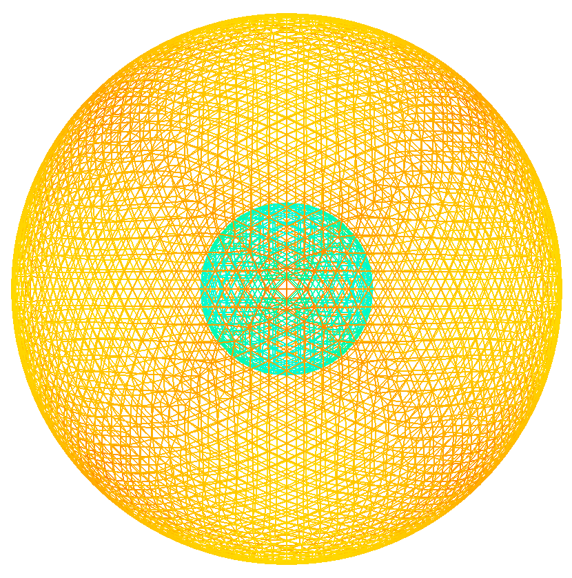
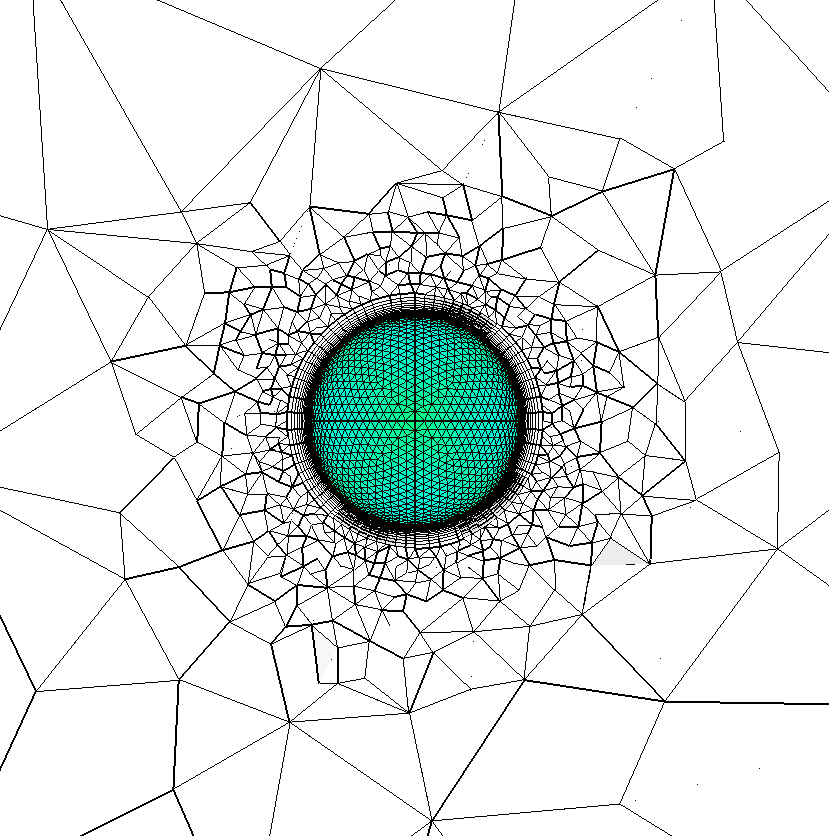
BL and spacing control. CFD applications often involve an outer
far-field surface that is much larger than the configuration of interest.
Further, the spacing on the outer boundary can often be increased considerably
as long as resolution is maintained near the configuration of interest. Here we
consider an extreme case, in terms of far-field coarseness, with an inner
sphere of radius 1 and an outer far-field of radius 20. The coarse far-field
impacts the near-field region around the inner sphere.
aflr3 -i spheres_1_20 -blc -blds 0.001 -blrm 1.2
If appropriate grid boundary conditions are not set in the input surface mesh
file then option flags can be used to specify appropriate values. See
documentation for more information on grid boundary condition values. Option
flags can be added to set the grid boundary condition flag for all surfaces.
For this case the inner sphere is ID=1 and the outer sphere is ID=3. Note that
the -bls option list only contains one ID and must be terminated with a comma.
The -bls option turns all other surfaces into non-BL generating surfaces so
that it is not necessary to set the BC on the outer sphere.
aflr3 -i spheres_1_3_20 -blc -blds 0.001 -blrm 1.2 -bls 1,
To lessen the impact of the far-field spacing a control surface can be
placed around the configuration of interest. The intent is simply to provide
more control of the near-field spacing. AFLR3 allows surfaces to define
sources with a spacing value derived from the surface itself. Individual points
with a spacing value could also be used. These surfaces are embedded or
transparent surfaces called source surfaces. A source surfaces can
intersect itself or other surfaces (of any kind) and even extend outside the
domain. Only the points on the surface that can be inserted into the domain and
are a sufficient distance from other points are retained. Unlike a true
embedded or transparent surface they will not interfere with the BL region. A
control source surface of a sphere with a radius of 3 is inserted into the
domain of the previous case to control the near-field spacing.
aflr3 -i spheres_1_3_20 -blc -blds 0.001 -blrm 1.2
If appropriate grid boundary conditions are not set in the input surface mesh
file then option flags can be used to specify appropriate values. See
documentation for more information on grid boundary condition values. Option
flags can be added to set the grid boundary condition flag for all
surfaces. Here a Grid_BC value of -1 denotes a BL generating solid surface
and a value of 3 denotes a source surface that is deleted after the points are
inserted and spacing values derived from the surface are set. For this case the
inner sphere is ID=1, the spacing control source surface is ID=2, and the outer
sphere is ID=4.
aflr3 -i spheres_1_3_20 -blc -blds 0.001 -blrm 1.2 -BC_IDs
1,2,4 -Grid_BC_Flag -1,3,1
BL parameters. Previous cases have all used the -blds parameter to set
the initial normal spacing. For turbulent flow CFD applications it is often
convenient to base the initial normal spacing in the BL region on the desired
initial y+ value and Reynolds number. For the previous case the initial spacing
of 0.001 corresponds to a y+ of 1.3 at a Reynolds number of 20,000 per grid
unit. The reference length chosen to set the evaluation Reynolds number is 1
grid unit. When using the physical BL parameters to set the initial spacing it
is useful to pre-check the actual spacing and parameters derived before generating
the mesh. Adding the -blcheck option outputs only the BL parameters and
performs initial checks without generating any mesh.
aflr3 -i spheres_1_3_20 -blc -Re 20000 -refx 1 -y+ 1.3 -blrm
1.2 -blcheck
The estimated BL thickness can also be set if set to a value of 0 using the
-bldel option. By default the BL thickness is set to -1 meaning it will not be
used or calculated.
aflr3 -i spheres_1_3_20 -blc -Re 20000 -refx 1 -y+ 1.3 -blrm
1.2 -bldel 0 -blcheck
The physical BL thickness may be less than or greater than the thickness
required for the BL region to grow the normal spacing to a value equal to the
surface tangential spacing. Adding the -bldelmax will compute and set the BL
thickness to the maximum of the physical value and the value needed to grow the
BL normal spacing to isotropic size.
aflr3 -i spheres_1_3_20 -blc -Re 20000 -refx 1 -y+ 1.3 -blrm
1.2 -bldelmax -blcheck
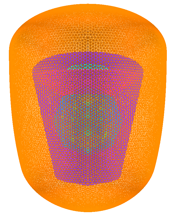
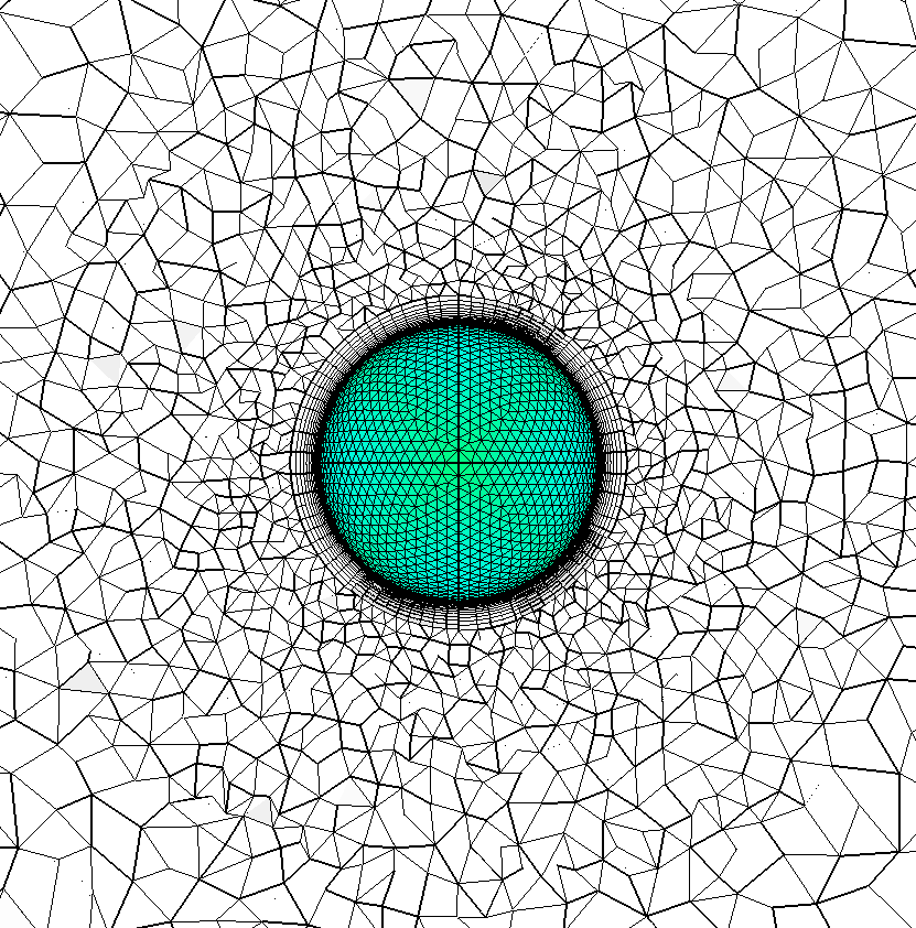
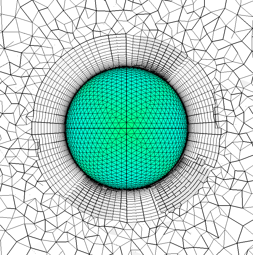
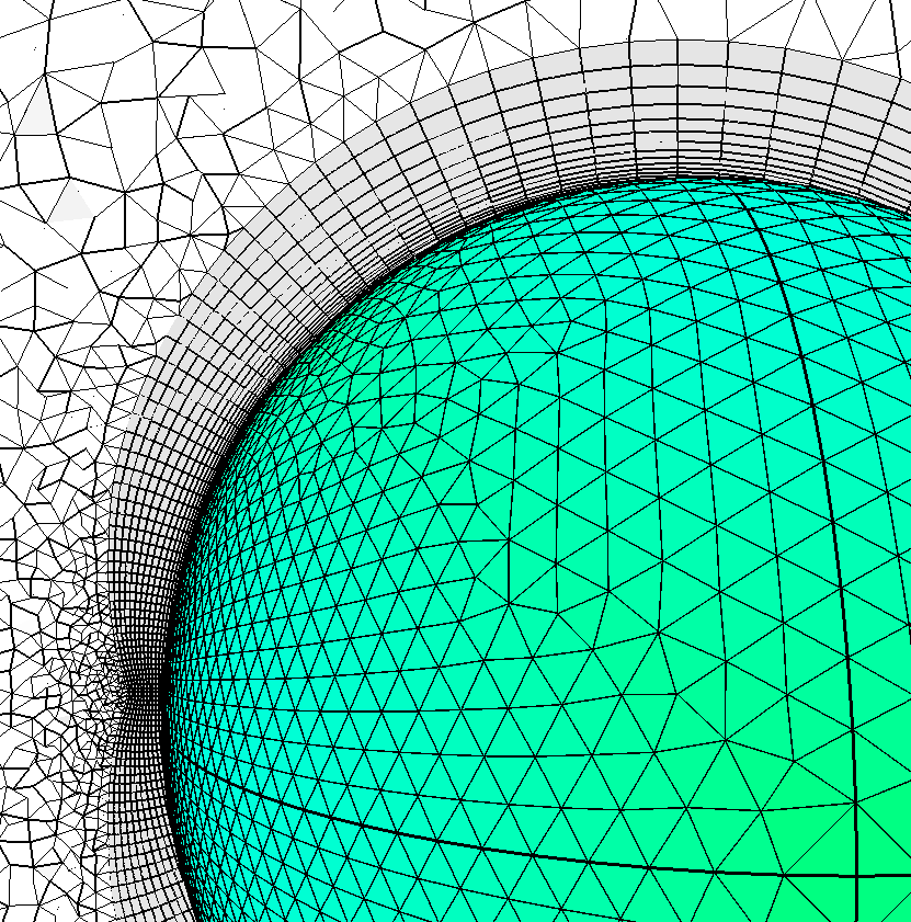
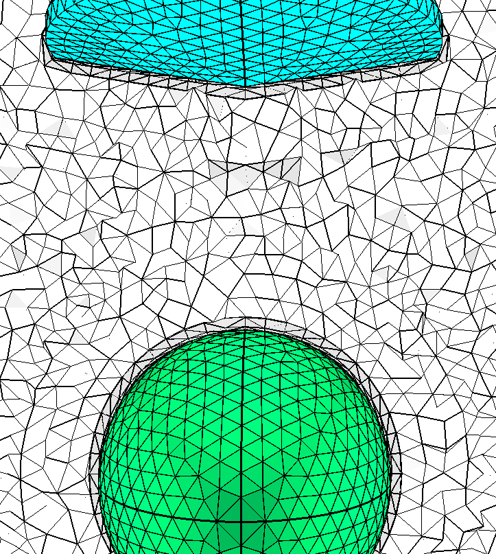
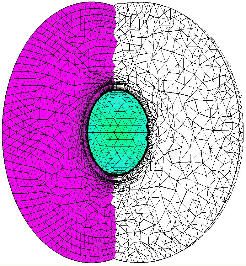
The previous case (with a control source surface) produces the following BL
region.
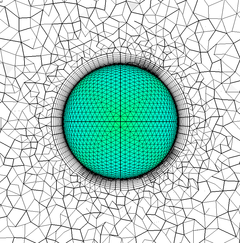
If a larger BL thickness is desired a value can be specified. Here we use the
-bldel option to choose a BL thickness of 0.5.
aflr3 -i spheres_1_3_20 -blc -blds 0.001 -blrm 1.2 -bldel
0.5
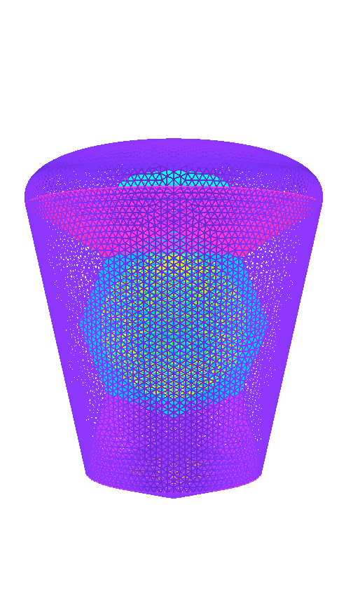
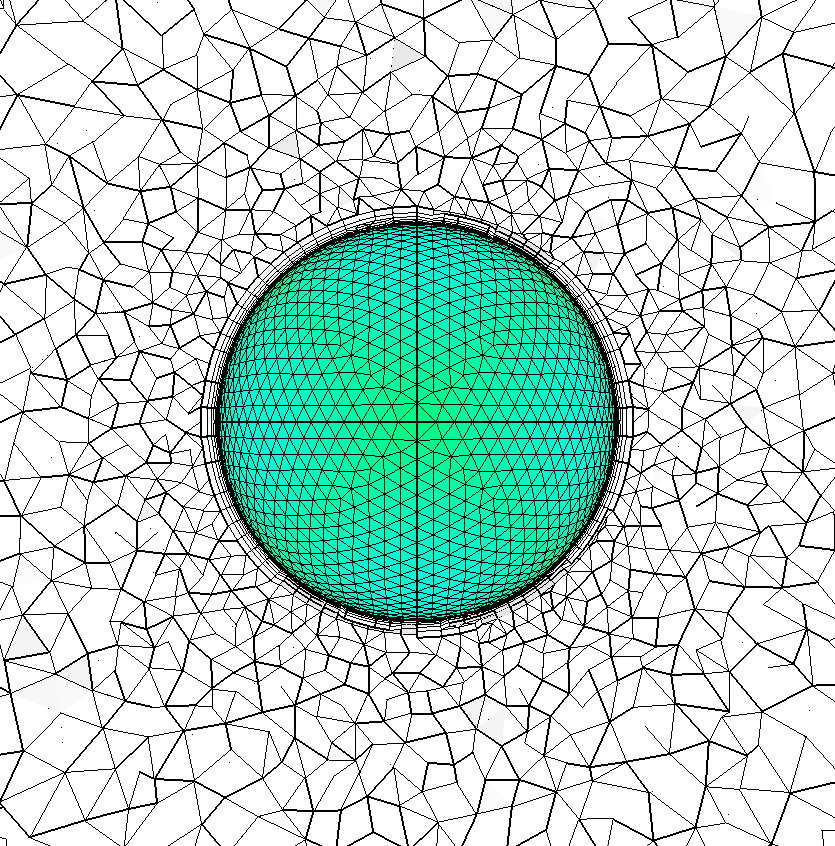
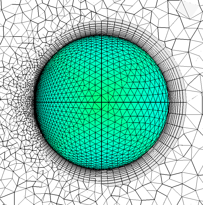
If we rerun with default BL growth (1.5) and with no BL thickness then
typically a relatively thin BL region is produced.
aflr3 -i spheres_1_3_20 -blc -blds 0.001
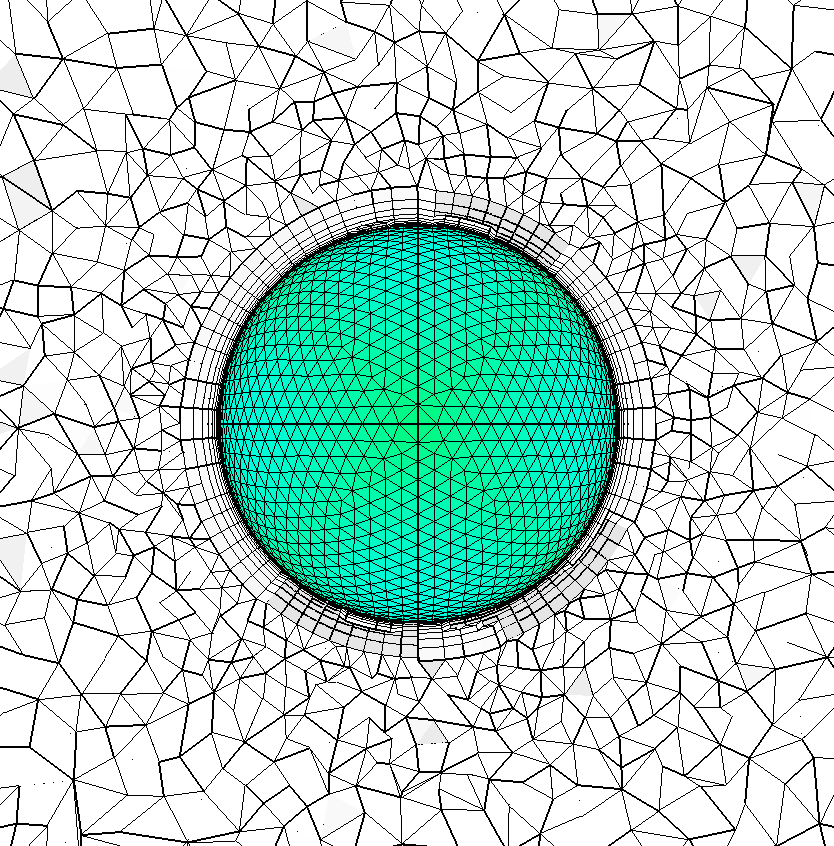
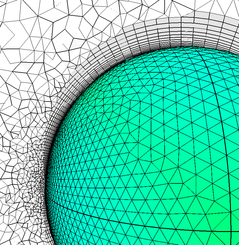
The previous case terminates when the normal spacing to tangential spacing
ratio is 0.5 (defined by cblmnr). If we set cblmnr to 0.9 the BL region will
grow further. A lower BL growth will also produce a thicker BL region. However,
it is usually set based on the accuracy needed in the BL region.
aflr3 -i spheres_1_3_20 -blc -blds 0.001 cblmnr=0.9
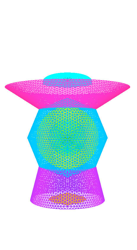
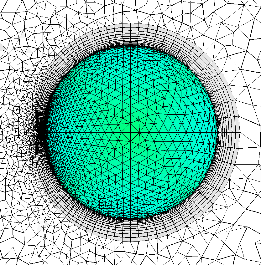
In the previous cases the surface spacing is uniform on the BL generating
surfaces. If the surface spacing varies then BL termination can vary locally or
be determined globally. By default BL termination is determined with a global
influence. The mblend option (mblend=1 is the default) can be used to toggle
between global and local termination. If we vary the spacing on the surface of
the inner sphere with the current case the resulting BL is relatively uniform
in number of layers. When the normal spacing for a particular location reaches
isotropic size then the BL doesn't necessarily terminate with global
termination. Instead advancement continues on at the maximum allowable normal
spacing for the particular location. However, this is not strictly enforced.
Merging BL regions, element quality and tangential size (above the surface in
the BL region) can terminate the BL advancement locally. In previous cases the
issue of local versus global termination was not relevant since the surface
spacing is uniform and all locations reach a normal spacing value equal to the
isotropic termination value (boundary surface tangential size) at the same
layer. The variable spacing version of the current case produces a relatively
uniform number of layers generated with global termination.
aflr3 -i spheres_1_3_20_vs -blc -blds 0.001 -blrm 1.2
With local termination (-mblend 0 or mblend=0 option) the number of layers
generated in the BL region varies locally and is dependent upon the local
surface tangential spacing.
aflr3 -i spheres_1_3_20_vs -blc -blds 0.001 -blrm 1.2
mblend=0
Note that if a large BL thickness is specified, e.g. -bldel 0.5, then the
differences will be minimized as that constraint can cause the BL region to
grown beyond the isotropic size (with constant normal spacing).
Nozzle with inlet and outlet. Inlet and outlet are treated as surfaces
that intersect the BL region and are rebuilt within AFLR3. The surface
grid on the nozzle wall is made up entirely of quad faces. Hex elements can be
generated in the BL region to reduce overall element count. The -blc3 option is
added to generate hex elements with pyramid element transition. Use of the
-blc2 option instead would generate hex elements with split face transition to
the tetrahedral isotropic mesh region. The maximum growth rate in the BL region
is limited to 1.2. This results in additional BL region resolution with a
typically greater extent. Note that appropriate grid boundary conditions are
set within the surface grid file.
aflr3 -i nozzle -blc3 -blds 0.0001 -blrm 1.2
If the input surface mesh does not contain grid boundary conditions then they
can be completely specified on the command line using option flags as shown
below. A TAGS file could also be used to set this information. For this case
the inlet and outlet rebuild surfaces are ID=1 and ID=2; and the BL generating
nozzle wall surface is ID=3. Note that the -bls option list only contains one
ID and must be terminated with a comma.
aflr3 -i curved_duct -blc -blds 0.00003 -bls 3, -ints 1,2
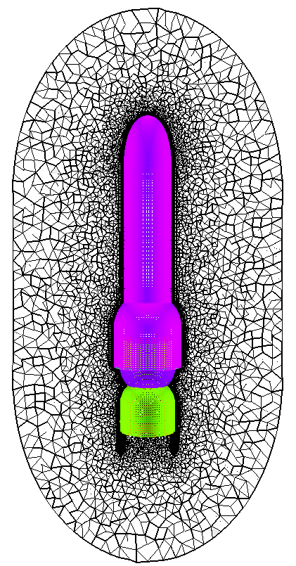
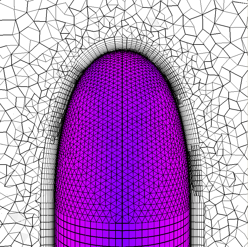
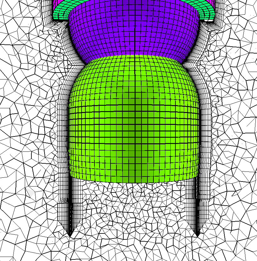
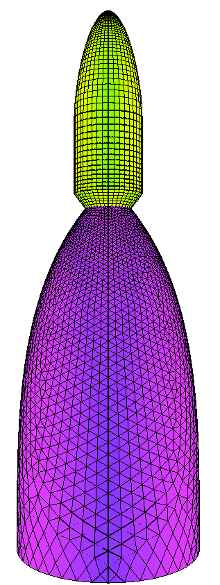
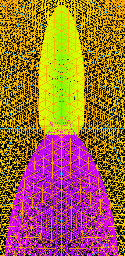
Rocket with engine, nozzle, plume and transparent internal data surfaces.
The rocket body, engine, and nozzle are treated as normal solid surfaces with
attached BL regions. The overall domain is enclosed in an outer boundary that
is relatively close to the Rocket simply to keep the domain size smaller.
Physics and solver may dictate otherwise. The plume is modeled as an
embedded/transparent delete surface with attached BL region. It is used to
generate a plume BL region and the plume surface connectivity description is
then deleted in the final volume mesh. Note that the plume ends close to, but
within, the outer boundary. It can not extend to the outer boundary as that
would create two completely separate domains for the tetrahedral interior
volume. If that is required then this case would need to be separated into two
separate domains. With one being inside the engine, nozzle and plume region.
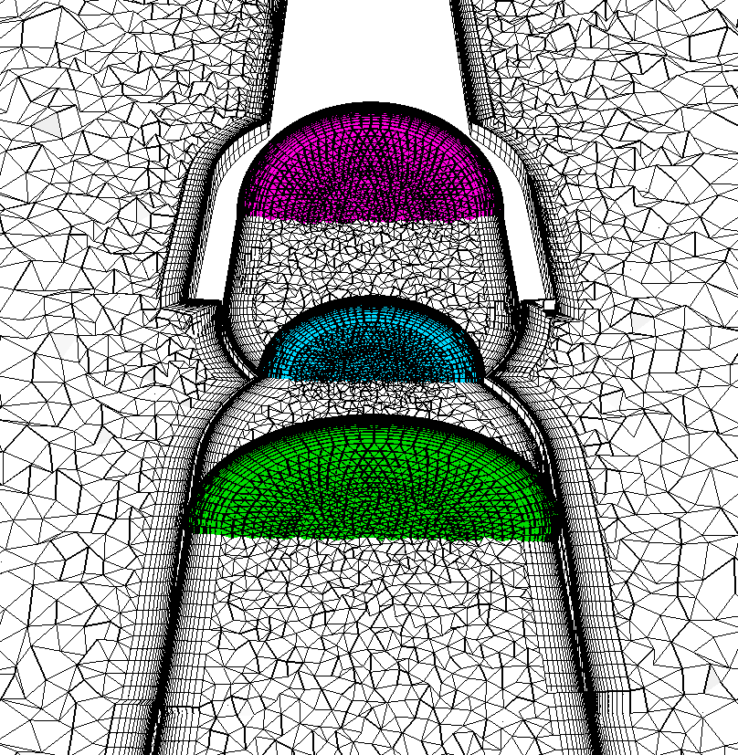
The internal engine inlet is treated as a surface that intersect the BL region
and is rebuilt within AFLR3. Internal data surfaces are placed at the
engine exit and near the nozzle exit. These are intended as simply surface on
which to collect data at known locations. They are treated as transparent
surfaces that intersect the BL region and are rebuilt within AFLR3.
Their connectivity is retained in the final volume mesh. Much of the surface
mesh contains quad faces and hex elements can be generated in the BL region to
reduce overall element count. The -blc3 option is added to generate hex
elements with pyramid element transition. Use of the -blc2 option instead would
generate hex elements with split face transition to the tetrahedral isotropic
mesh region. The maximum growth rate in the BL region is limited to 1.2. This
results in additional BL region resolution with a typically greater extent.
Note that appropriate grid boundary conditions are set within the surface grid
file.
aflr3 -i rocket -blc3 -blds 0.0001 -blrm 1.2
If the input surface mesh does not contain grid boundary conditions then they
can be completely specified on the command line using option flags as shown
below. A TAGS file could also be used to set this information. Here a Grid_BC
value of -1 denotes a BL generating solid surface, a value of 1 denotes a
standard surface, a value of 2 denotes a surface that intersects the BL region
and that is rebuilt by AFLR3, a value of 4 denotes an
embedded/transparent surface that intersects the BL region and that is rebuilt
by AFLR3, and a value of -6 denotes an embedded/transparent delete
surface that generates a BL mesh on both sides. For this case the outer
boundary is ID=1; the inlet and rebuild surface is ID=4; the engine and nozzle
exhaust internal rebuild surfaces are ID=6 and ID=16; the plume and internal BL
generating surface is ID=2, and the BL generating missile, engine, and nozzle
wall surfaces are ID=3, ID=5, ID=7, ID=8, ID=9, and ID=10.
aflr3 -i rocket -blc3 -blds 0.0001 -blrm 1.2 -BC_IDs
1,2,3,4,5,6,7,8,9,10,16 \
-Grid_BC_Flag 1,-6,-1,2,-1,4,-1,-1,-1,-1,4
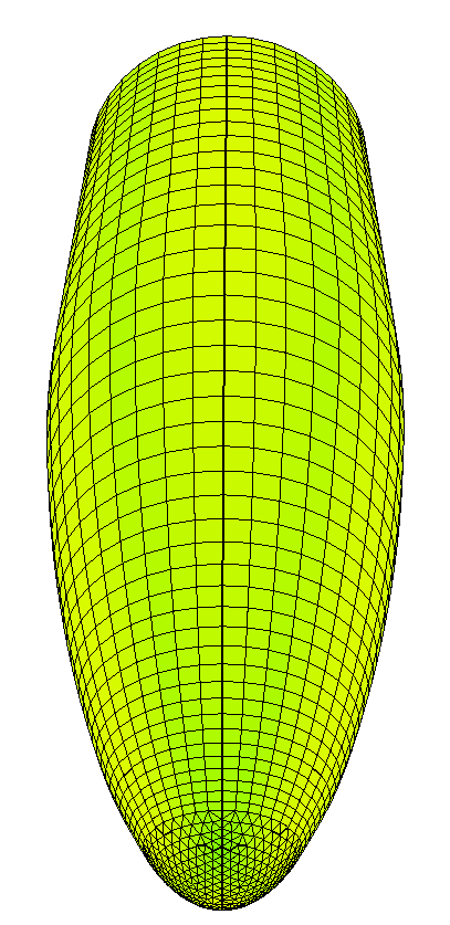
Open BL mesh closed domain for a rocket with engine, nozzle and transparent
internal data surfaces. An open BL mesh (and closed domain) can be
generated for the previous case with the -open option. With an open BL mesh
(and closed domain) the final volume mesh will be composed of only BL region
volume elements. All surfaces are retained in the output mesh. The interior
tetrahedral elements will not be generated. All surfaces that intersect the BL
region will be conformed to as normal. Transparent surfaces that are set to
generate a BL region will be treated as normal. Open BL open domain
configurations must be fully closed (unless transparent) in the same manner as
with AFLR3 in normal mode.
aflr3 -i rocket -blc3 -blds 0.0001 -blrm 1.2 -open
If the input surface mesh does not contain grid boundary conditions then they
can be completely specified on the command line using option flags as shown
below. Note that here we are inputing the entire surface mesh so BCs are needed
for those that won't be included.
aflr3 -i rocket -blc3 -blds 0.0001 -blrm 1.2 -open -BC_IDs
1,2,3,4,5,6,7,8,9,10,16 \
-Grid_BC_Flag 1,-6,-1,2,-1,4,-1,-1,-1,-1,4
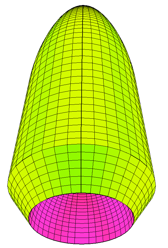
Open BL mesh open domain for a rocket with engine, nozzle and transparent
internal data surfaces. An open BL mesh (and open domain) can be generated
for the previous case with the -open2 option. Such a mesh could be used in an
oversee type application. With an open BL mesh the final volume mesh will be
composed of only BL region volume elements. Only the solid BL generating
surfaces are retained. The interior tetrahedral elements will not be generated.
All surfaces that intersect the BL region will be conformed to as normal.
Transparent surfaces that are set to generate a BL region will be ignored. Open
BL configurations can be defined with open surfaces that would not be valid for
a normal mesh generation case . For example, a wing by itself would be valid
for an open BL open domain case. If any of the surfaces are open the BL mesh
will be generated without constraint using a normal determined from the
boundary surface. If there is any curvature near the open end then open end BL
mesh will be non-planar (it would be planar for an open tube). The direction of
the BL normal is not unique in the open domain case and a BL region may be
generated on either side of a surface. If the surfaces have a consistent
ordering then at most one needs to do is reverse the direction using the option
(-revbl). For the rocket case the normals must be reversed to be in the correct
direction so the -revbl option must be used with the -open2 option. If a
configuration contains multiple surfaces and they are not consistently ordered
then reordering by another procedure is required.
aflr3 -i rocket -blc3 -blds 0.0001 -blrm 1.2 -open2
-revbl
If the input surface mesh does not contain grid boundary conditions then they
can be completely specified on the command line using option flags as shown
below. Note that here we are inputing the entire surface mesh so BCs are needed
for those that won't be included.
aflr3 -i rocket -blc3 -blds 0.0001 -blrm 1.2 -open2 -revbl
-BC_IDs 1,2,3,4,5,6,7,8,9,10,16 \
-Grid_BC_Flag 1,-6,-1,2,-1,4,-1,-1,-1,-1,4
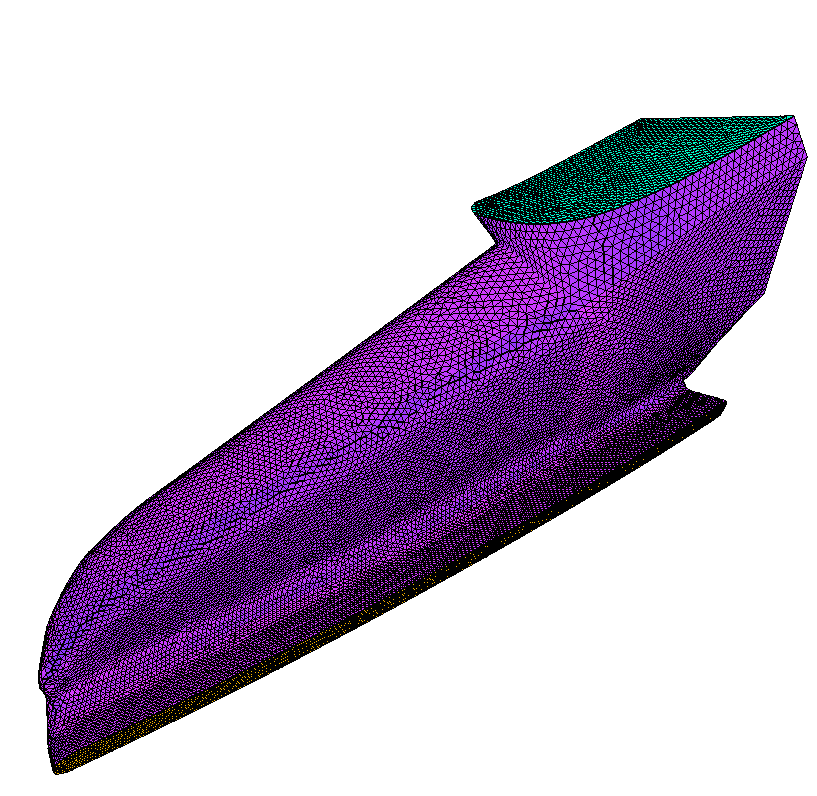
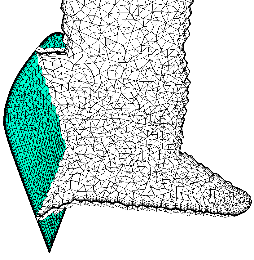
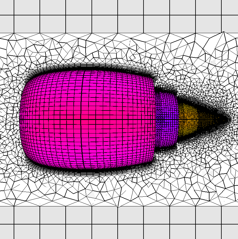
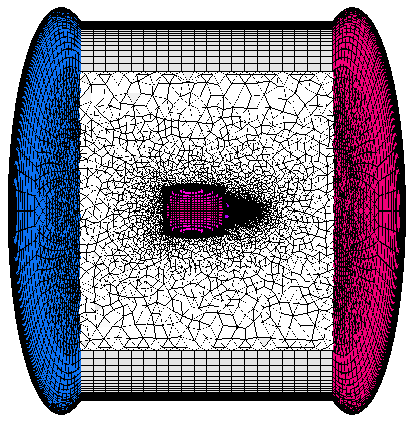
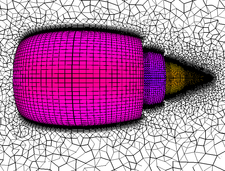
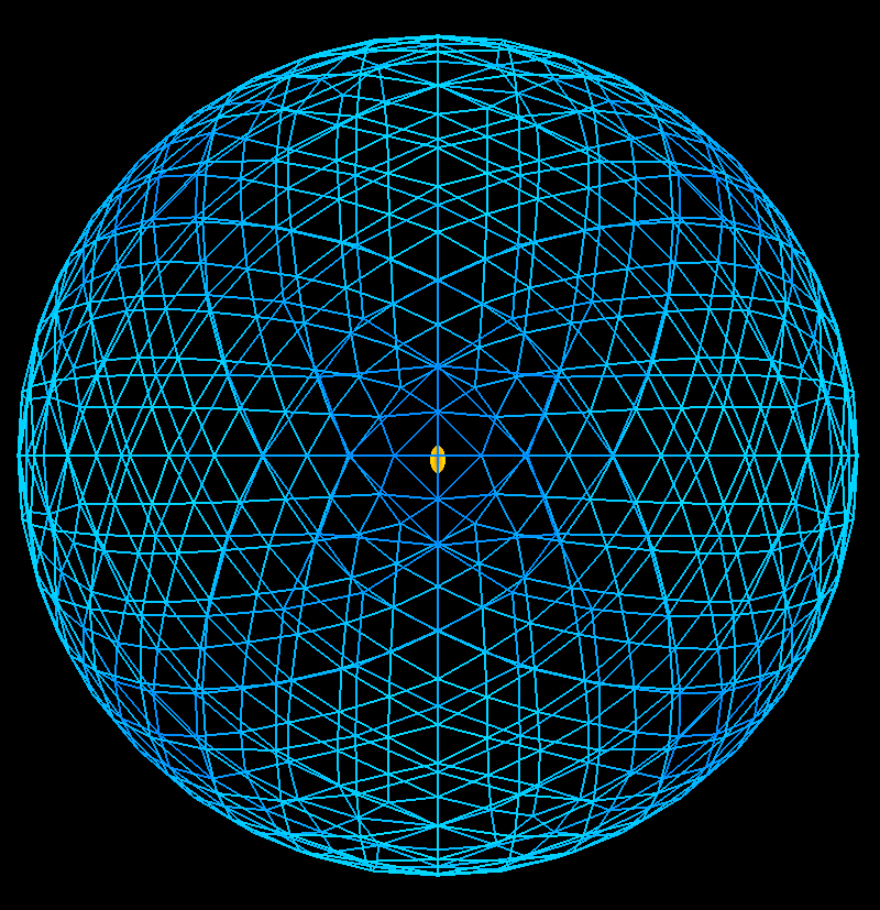
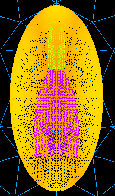
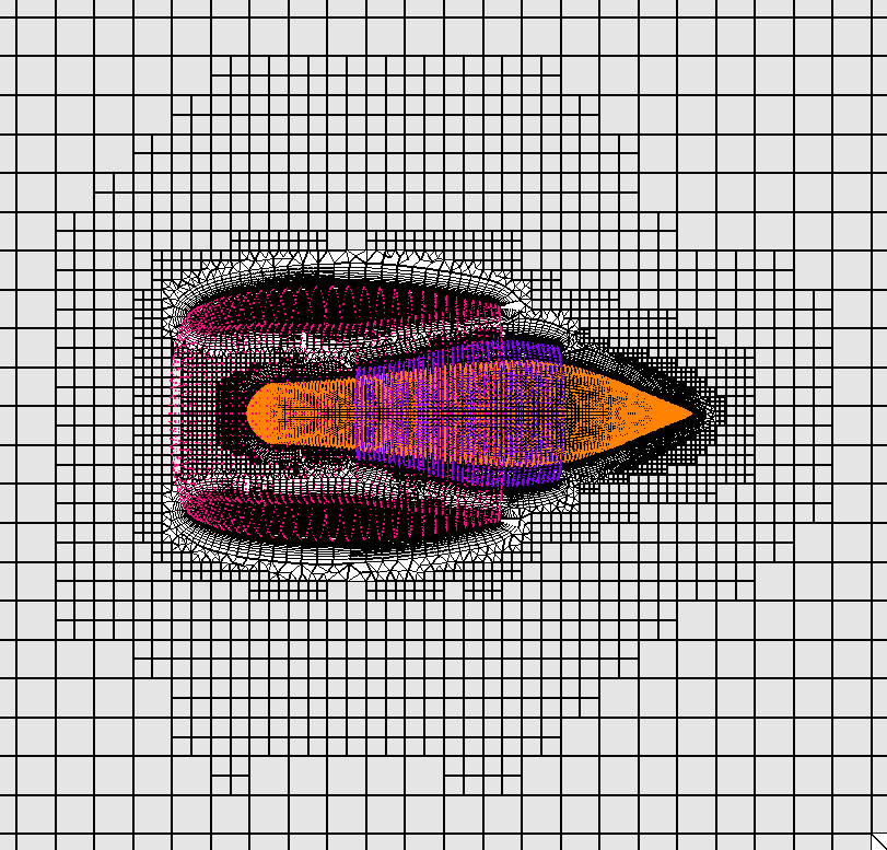
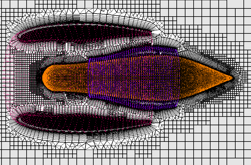
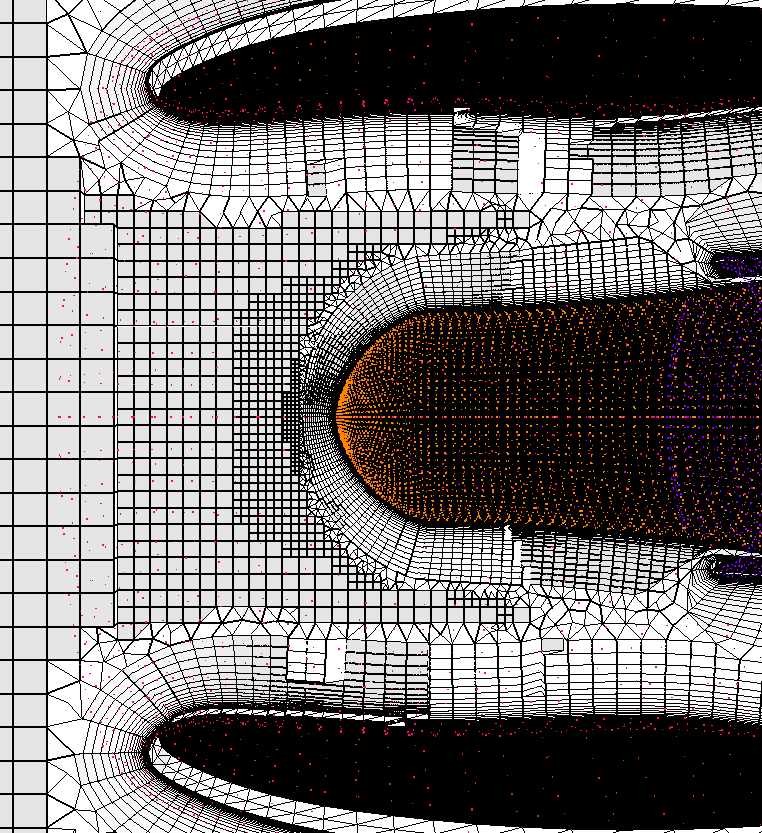
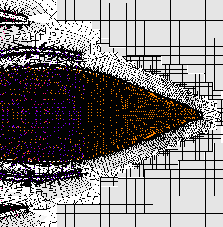
Missile with nozzle, plume and near-field control surface. The
near-field control surface is modeled as an embedded/transparent source
surface. A transparent source surface is simply used to control spacing nearby.
The source surface provides a means of determining the appropriate local length
scale. Outside of the source surface the element size increases relatively
rapidly with growth out to the very coarse far-field. Note that with an
embedded/transparent source surface only the surface points are inserted into
the volume mesh. If any of those points do not lie in the volume mesh region
they are ignored. The plume is modeled as an embedded/transparent delete
surface with attached BL region. It is used to generate the plume BL region and
the plume surface connectivity description is then deleted in the final volume
mesh. Note that transparent and transparent delete surfaces must be fully
enclosed within the domain and not intersect another surface. They are treated
the same as any other domain surface within AFLR3. A nozzle inlet is
included that is treated as a surface that intersects the BL region and is
rebuilt within AFLR3. Much of the surface mesh contains quad faces and
hex elements can be generated in the BL region to reduce overall element count.
The -blc3 option is added to generate hex elements with pyramid element
transition. Note that appropriate grid boundary conditions are set within the
surface grid file.
aflr3 -i missile1 -blc3 -blds 0.0001

If the input surface mesh does not contain grid boundary conditions then they
can be completely specified on the command line using option flags as shown
below. A TAGS file could also be used to set this information. Here a Grid_BC
value of -1 denotes a BL generating solid surface, a value of 1 denotes a
standard surface, a value of 2 denotes a surface that intersects the BL region
and that is rebuilt by AFLR3, a value of 3 denotes an
embedded/transparent source surface, and a value of -6 denotes an
embedded/transparent delete surface that generates a BL mesh on both sides. For
this case the outer boundary is ID=6; the nozzle inlet and rebuild surface is
ID=1; the spacing control source surface is ID=2, the plume and internal BL
generating surface is ID=3, and the BL generating missile and nozzle wall
surfaces are ID=4 and ID=5.
aflr3 -i missile1 -blc3 -blds 0.0001 -blrm 1.2 -BC_IDs
1,2,3,4,5,6 -Grid_BC_Flag 2,3,-6,-1,-1,1
Use of the -blc2 option instead generates hex elements with split face
transition to the tetrahedral isotropic mesh region. The BL region remains
largely the same. However the interior tetrahedral region will differ slightly
due to the split face transition.
aflr3 -i missile1 -blc2 -blds 0.0001
Missile with nozzle, plume, near-field control surface, and symmetry plane. This
case is exactly the same as the previous case, except that it is split into two
halves and a symmetry plane is added.
aflr3 -i missile2 -blc3 -blds 0.0001
If the input surface mesh does not contain grid boundary conditions then they
can be completely specified on the command line using option flags as shown
below. A TAGS file could also be used to set this information. Here a Grid_BC
value of -1 denotes a BL generating solid surface, a value of 1 denotes a
standard surface, a value of 2 denotes a surface that intersects the BL region
and that is rebuilt by AFLR3, a value of 3 denotes an
embedded/transparent source surface, and a value of -6 denotes an
embedded/transparent delete surface that generates a BL mesh on both sides. For
this case the outer boundary is ID=1; the nozzle inlet and rebuild surface is
ID=6; the spacing control source surface is ID=5, the plume and internal BL
generating surface is ID=4, the BL generating missile and nozzle wall surfaces
are ID=2 and ID=3; and the near-field and far-field symmetry surfaces are ID=7
and ID=8. Not that only the near-field symmetry surfaces needs to be rebuilt.
aflr3 -i missile2 -blc3 -blds 0.0001 -blrm 1.2 -BC_IDs
1,2,3,4,5,6,7,8 \
-Grid_BC_Flag 1,-1,-1,-6,3,2,1,2
Missile with nozzle, plume and symmetry plane. This case is a subset of
the previous case, except that the outer boundary is removed. The domain is now
truncated at what was the near-field control surface which is now the outer
boundary and treated as a standard surface. Note that appropriate grid boundary
conditions are set within the surface grid file.
aflr3 -i missile3 -blc3 -blds 0.0001

If the input surface mesh does not contain grid boundary conditions then they
can be completely specified on the command line using option flags as shown
below. A TAGS file could also be used to set this information. Here a Grid_BC
value of -1 denotes a BL generating solid surface, a value of 1 denotes a
standard surface, a value of 2 denotes a surface that intersects the BL region
and that is rebuilt by AFLR3, and a value of -6 denotes an
embedded/transparent delete surface that generates a BL mesh on both sides. For
this case the outer boundary is ID=3; the nozzle inlet and rebuild surface is
ID=2; the plume and internal BL generating surface is ID=4; the BL generating
missile and nozzle wall surfaces are ID=5 and ID=6; and the symmetry surface is
ID=1.
aflr3 -i missile3 -blc3 -blds 0.0001 -blrm 1.2 -BC_IDs
1,2,3,4,5,6 -Grid_BC_Flag 2,2,1,-6,-1,-1
This information can be set in the TAGS file. Addition of the -tags option causes
AFLR3 to search for a file named missile3.tags. If found then it is read
and all grid boundary condition related parameters are reset to those in the
TAGS file from default or those specified in the input surface mesh file. Note
that most of the example cases are provided with appropriate TAGS files.
aflr3 -i missile3 -blc3 -blrm 1.2 -blds 0.0001 -tags
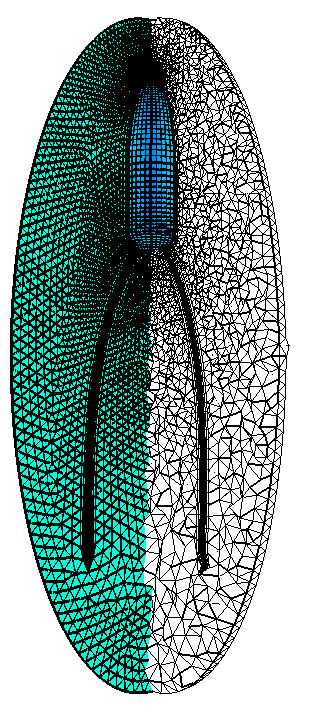
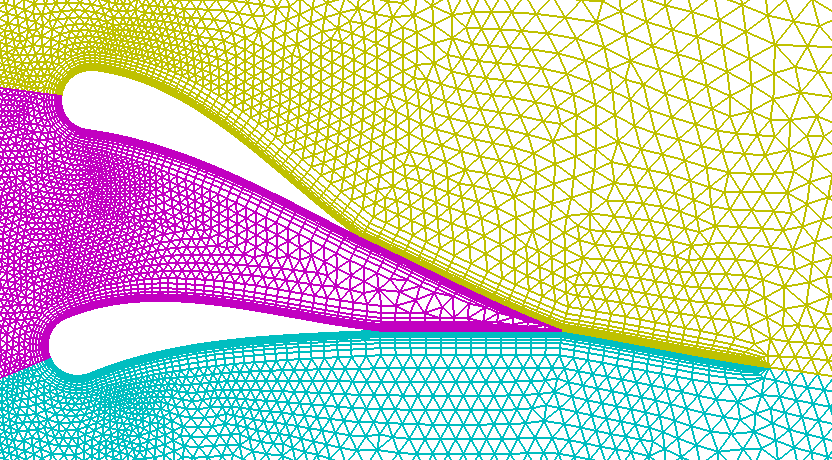
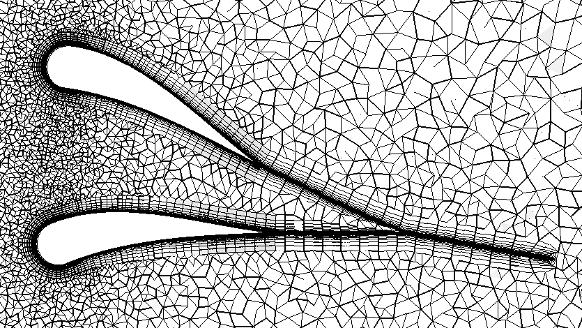
Two blades with merging wakes and symmetry plane. The two blades are
treated as normal solid surfaces with attached BL regions. The overall domain
is enclosed in an outer boundary. Physics and solver may dictate a differing
size of outer boundary. The wake region is modeled as an embedded/transparent
delete surface with attached BL region. The wake surfaces are used to generate
a wake BL region from each blade that merges into a single wake. The
connectivity description for the wake surfaces are then deleted in the final
volume mesh. The maximum growth rate in the BL region is limited to 1.4. This
results in additional BL region resolution with a slightly greater extent. Note
that appropriate grid boundary conditions are set within the surface grid file.
Some of the surface mesh contains quad faces and hex elements can be generated
in the BL region to reduce overall element count. The -blc3 option is added to
generate hex elements with pyramid element transition. Use of the -blc2 option
instead would generate hex elements with split face transition to the
tetrahedral isotropic mesh region.
aflr3 -i two_blade_wake_sym -blc3 -blrm 1.4 -blds 0.0001
Note also that the BL region on the edges of the wakes ends abruptly. Ideally
the wake is extended to the outer boundary or the normal spacing is increased
along the wake up to a value approaching the isotropic element size. However,
this can can be difficult in either case and will result in additional mesh
points being generated. In particular to increase the normal spacing along the
wake up to isotropic size can take considerable distance to achieve without
resulting in element quality degradation due to the edge length growth rate
required.
If the input surface mesh does not contain grid boundary conditions then they
can be completely specified on the command line using option flags as shown
below. A TAGS file could also be used to set this information. Here a Grid_BC
value of -1 denotes a BL generating solid surface, a value of 1 denotes a
standard surface, a value of 2 denotes a surface that intersects the BL region
and that is rebuilt by AFLR3, and a value of -6 denotes an
embedded/transparent delete surface that generates a BL mesh on both sides. For
this case the BL generating blade wall surfaces are ID=5 and ID=4; the wake BL
generating surfaces are ID=3, ID=2 and ID=1; the symmetry surfaces are ID=35,
ID=34 and ID=33; and the outer boundaries are ID=36, ID=37, ID=38, ID=39,
ID=40, ID=42 and ID=43.
aflr3 -i two_blade_wake_sym -blc3 -blrm 1.4 -blds 0.0001 \
-BC_IDs 5,4,3,2,1,35,34,33,36,37,38,39,40,42,43 \
-Grid_BC_Flag -1,-1,-6,-6,-6,2,2,2,1,1,1,1,1,1,1
This information can be set in the TAGS file. Addition of the -tags option
causes AFLR3 to search for a file named two_blade_wake_sym.tags. If
found then it is read and all grid boundary condition related parameters are
reset to those in the TAGS file from default or those specified in the input
surface mesh file. Note that most of the example cases are provided with
appropriate TAGS files. Note that there may be slight differences in the output
mesh as the ordering can change slightly with a TAGS file.
aflr3 -i two_blade_wake_sym -blc3 -blrm 1.4 -blds 0.0001
-tags
Two blades with merging wakes, extended wake and symmetry plane. This
case is similar to the previous two blade example except that here the wake is
extended to the outer boundary. This eliminates the abrupt BL termination on
the end of the wake at the expense of additional mesh points. In this case the
increase in mesh points is about 6%. Note that the abrupt BL termination at the
edges on the side of the wake are still present. Note that appropriate grid
boundary conditions are set within the surface grid file. Some of the surface
mesh contains quad faces and hex elements can be generated in the BL region to
reduce overall element count. The -blc3 option is added to generate hex
elements with pyramid element transition. Use of the -blc2 option instead would
generate hex elements with split face transition to the tetrahedral isotropic
mesh region.
aflr3 -i two_blade_wake_sym_extended -blc3 -blrm 1.4 -blds
0.0001

If the input surface mesh does not contain grid boundary conditions then they
can be completely specified on the command line using option flags as shown
below. A TAGS file could also be used to set this information. Here a Grid_BC
value of -1 denotes a BL generating solid surface, a value of 1 denotes a
standard surface, a value of 2 denotes a surface that intersects the BL region
and that is rebuilt by AFLR3, and a value of -6 denotes an
embedded/transparent delete surface that generates a BL mesh on both sides. For
this case the BL generating blade wall surfaces are ID=5 and ID=4; the wake BL
generating surfaces are ID=3, ID=2 and ID=1; the symmetry surfaces are ID=35,
ID=34 and ID=33; , the outer rebuild surfaces that the wake intersects are
ID=42 and ID=43; and the outer boundaries are ID=36, ID=37, ID=38, ID=39 and
ID=40.
aflr3 -i two_blade_wake_sym_extended -blc3 -blrm 1.4 -blds
0.0001 \
-BC_IDs 5,4,3,2,1,41,35,34,33,42,43,36,37,38,39,40 \
-Grid_BC_Flag -1,-1,-6,-6,-6,-6,2,2,2,2,2,1,1,1,1,1
This information can be set in the TAGS file. Addition of the -tags option
causes AFLR3 to search for a file named two_blade_wake_sym.tags. If found
then it is read and all grid boundary condition related parameters are reset to
those in the TAGS file from default or those specified in the input surface
mesh file. Note that most of the example cases are provided with appropriate
TAGS files. Note that there may be slight differences in the output mesh as the
ordering can change slightly with a TAGS file.
aflr3 -i two_blade_wake_sym_extended -blc3 -blrm 1.4 -blds
0.0001 -tags
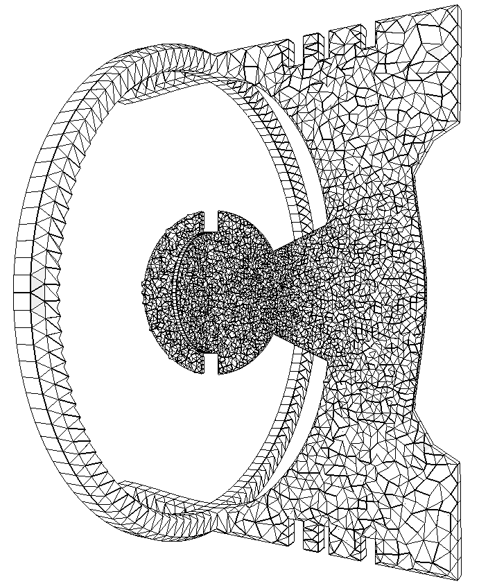
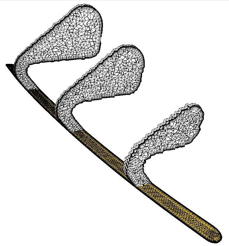
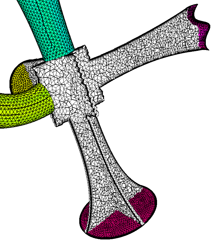
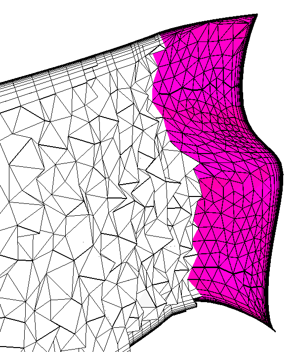
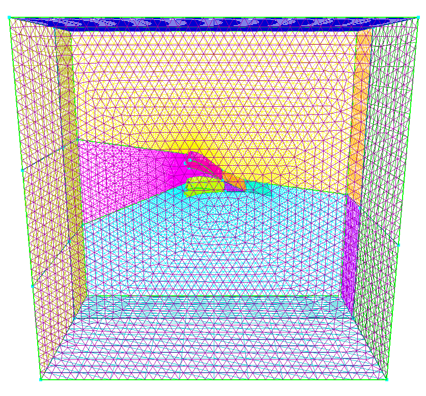
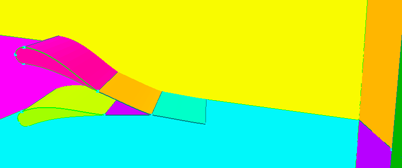
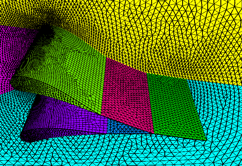
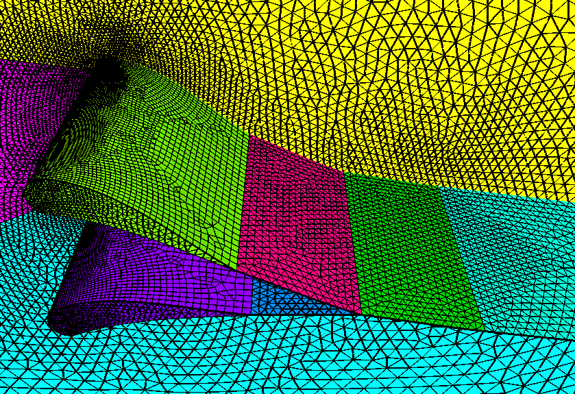
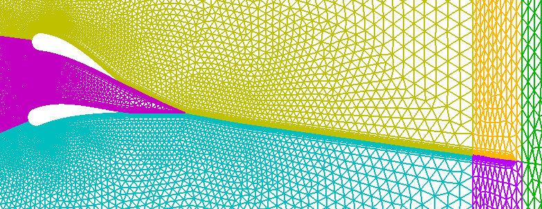
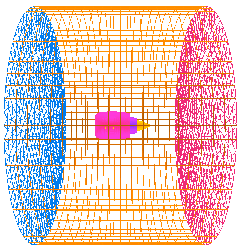
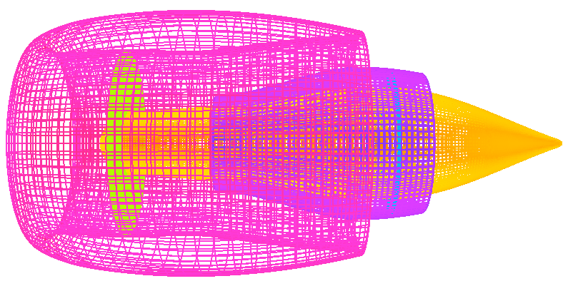
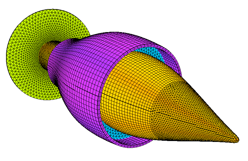
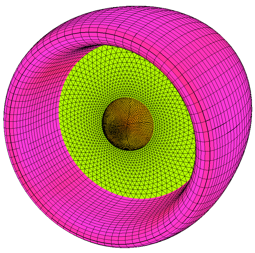
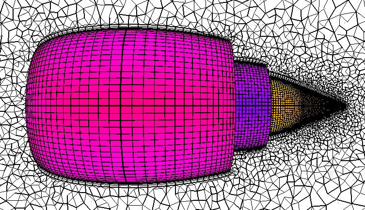
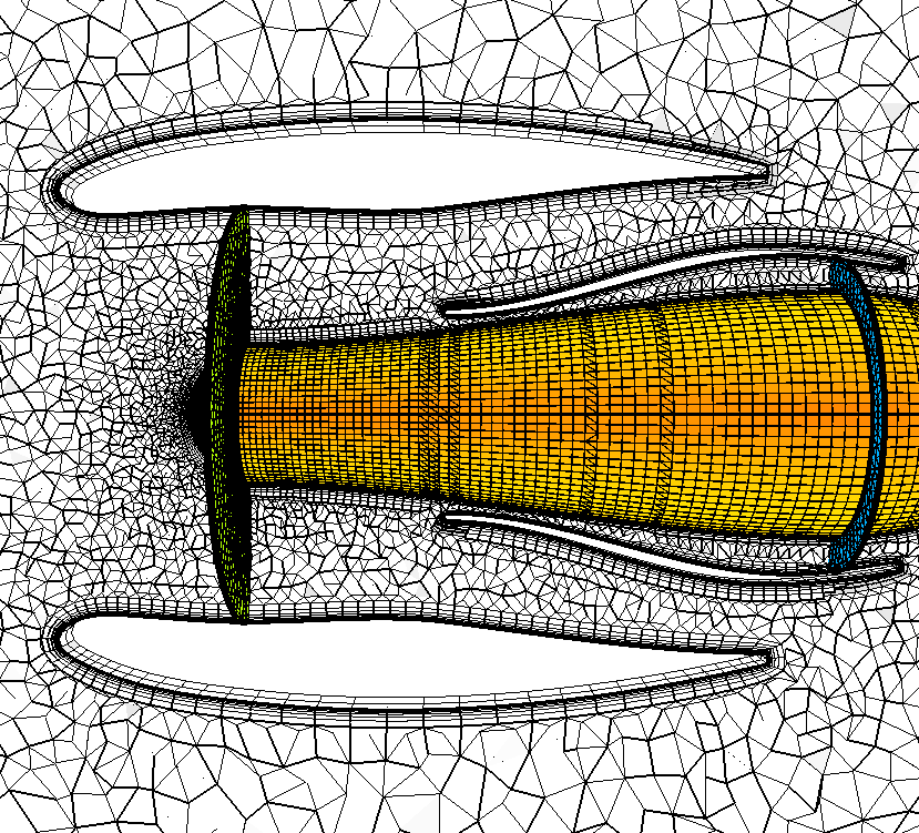
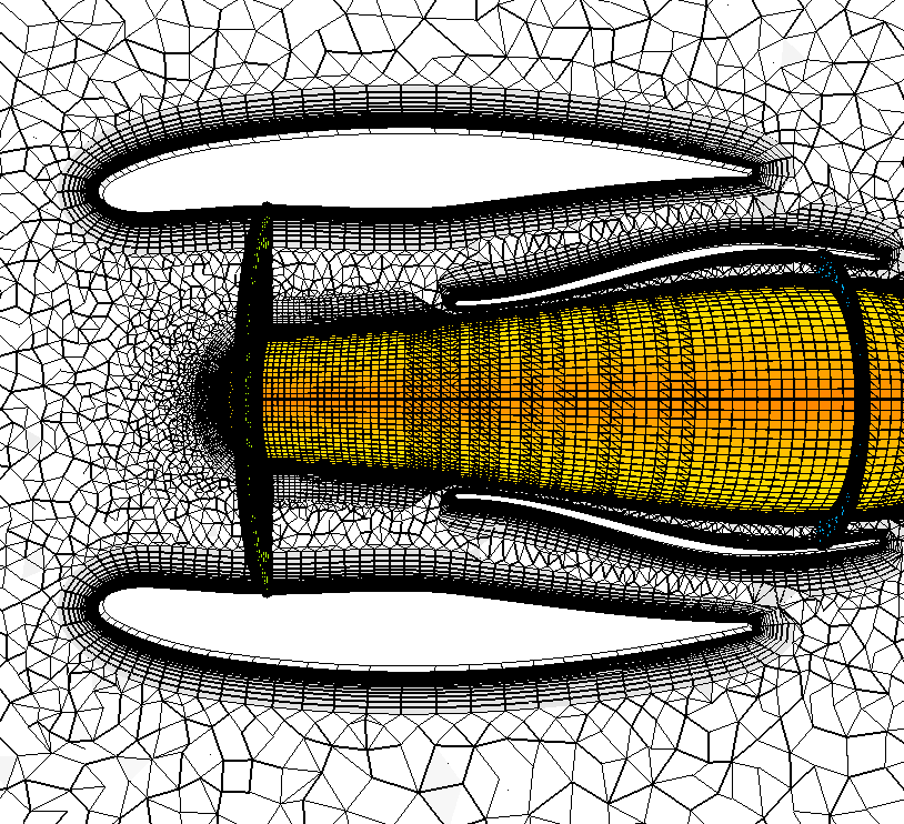
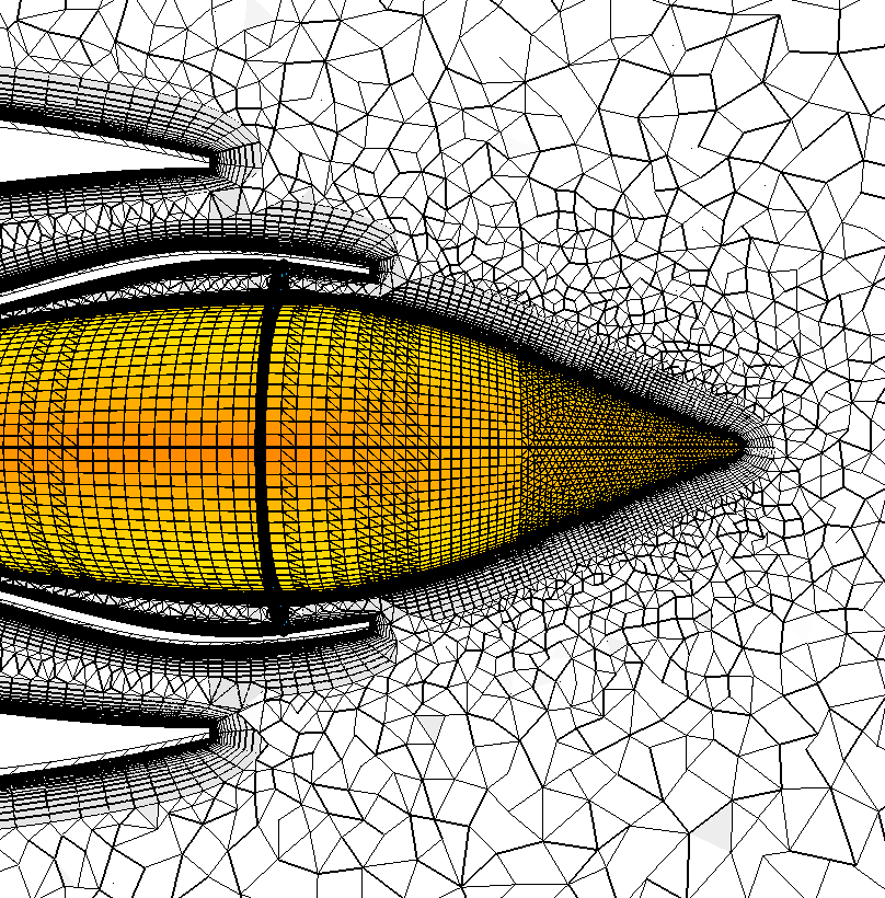
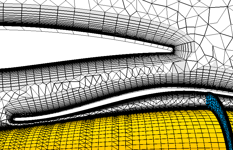
Aircraft nacelle with engine inside a section of wind tunnel. The
compressor fan and turbine blades are modeled with embedded/transparent
surfaces. Those surfaces along with the tunnel inlet and exit planes are
treated as surfaces that intersect the BL region and are rebuilt within AFLR3.
Note that appropriate grid boundary conditions are set within the surface grid
file. Much of the surface mesh contains quad faces and hex elements can be
generated in the BL region to reduce overall element count. The -blc3 option is
added to generate hex elements with pyramid element transition. Use of the
-blc2 option instead would generate hex elements with split face transition to
the tetrahedral isotropic mesh region.
aflr3 -i nacelle_engine -blc3 -blds 0.0002
For this case it may be desired to use a lower maximum growth rate (default is
1.5) in the BL and a coarser BL resolution on the tunnel wall. The -BL_IDs and
-BL_DS options can be added to modify the initial BL normal spacing for each
surface. The surface IDs specified below are the BL generating surfaces. In addition
a maximum BL growth rate of 1.2 is specified. For this case the tunnel inflow
and outflow rebuild surfaces are ID=11 and ID=12; the engine core, engine hub,
nacelle, and tunnel wall BL generating surfaces are ID=2, ID=3, ID=4, and ID-7,
and the fan disk and turbine disk internal rebuild surfaces are ID=5 and ID=6.
aflr3 -i nacelle_engine -blc3 -blrm 1.2 -BC_IDs 2,3,4,7
-BL_DS 0.0002,0.0002,0.0002,0.02
To reduce the number of BL region layers on the tunnel wall the -Number_of_BLs
option can be added. Setting the number of layers to 0 in this option flag
specifies that AFLR3 should choose the number of BL region layers to
generate for the corresponding surface ID.
aflr3 -i nacelle_engine -blc3 -blrm 1.2 -BC_IDs 2,3,4,7
-BL_DS 0.0002,0.0002,0.0002,0.02 \
-Number_of_BLs 0,0,0,44
If appropriate grid boundary conditions are not set in the input surface mesh
file then option flags can be used to specify appropriate values. Option flags
can be added to set the grid boundary condition flag, initial normal spacing
and number of BL region layers for all surfaces. See documentation for more
information on grid boundary condition values. Here a Grid_BC value of -1
denotes a BL generating solid surface, a value of 2 denotes a surface that
intersects the BL region and that is rebuilt by AFLR3, and a value of 4
denotes an embedded/transparent surface that intersects the BL region and that
is rebuilt by AFLR3. For this case the tunnel inflow and outflow rebuild
surfaces are ID=11 and ID=12; the engine core, engine hub, nacelle, and tunnel
wall BL generating surfaces are ID=2, ID=3, ID=4, and ID-7, and the fan disk
and turbine disk internal rebuild surfaces are ID=5 and ID=6.
aflr3 -i nacelle_engine -blc3 -blrm 1.2 -BC_IDs
2,3,4,5,6,7,11,12 \
-Grid_BC_Flag -1,-1,-1,4,4,-1,2,2 \
-Number_of_BLs 0,0,0,0,0,44,0,0 -BL_DS 0.0002,0.0002,0.0002,0,0,0.02,0,0
This information can be set in the TAGS file. Addition of the -tags option
causes AFLR3 to search for a file named nacelle_engine.tags. If found
then it is read and all grid boundary condition related parameters are reset to
those in the TAGS file from default or those specified in the input surface
mesh file. Note that most of the example cases are provided with appropriate
TAGS files.
aflr3 -i nacelle_engine -blc3 -blrm 1.2 -tags
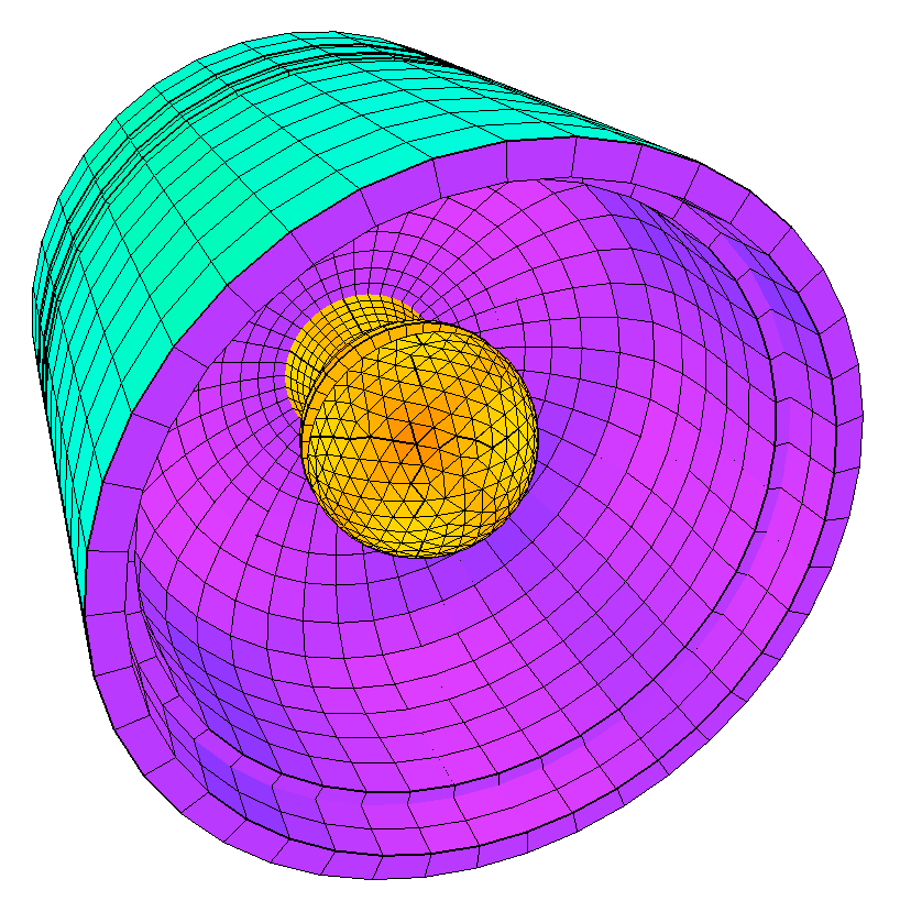
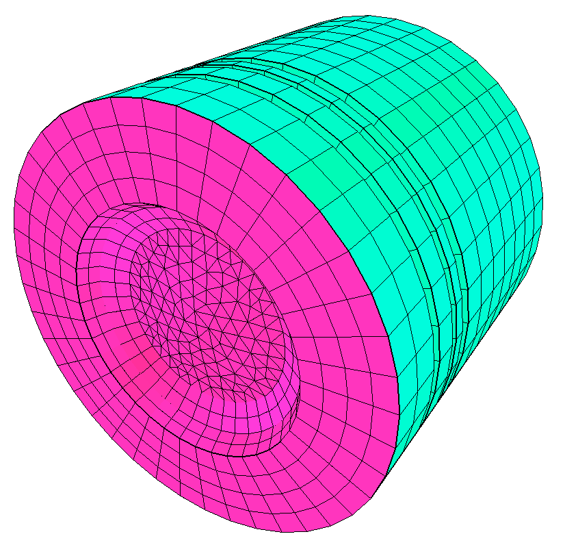
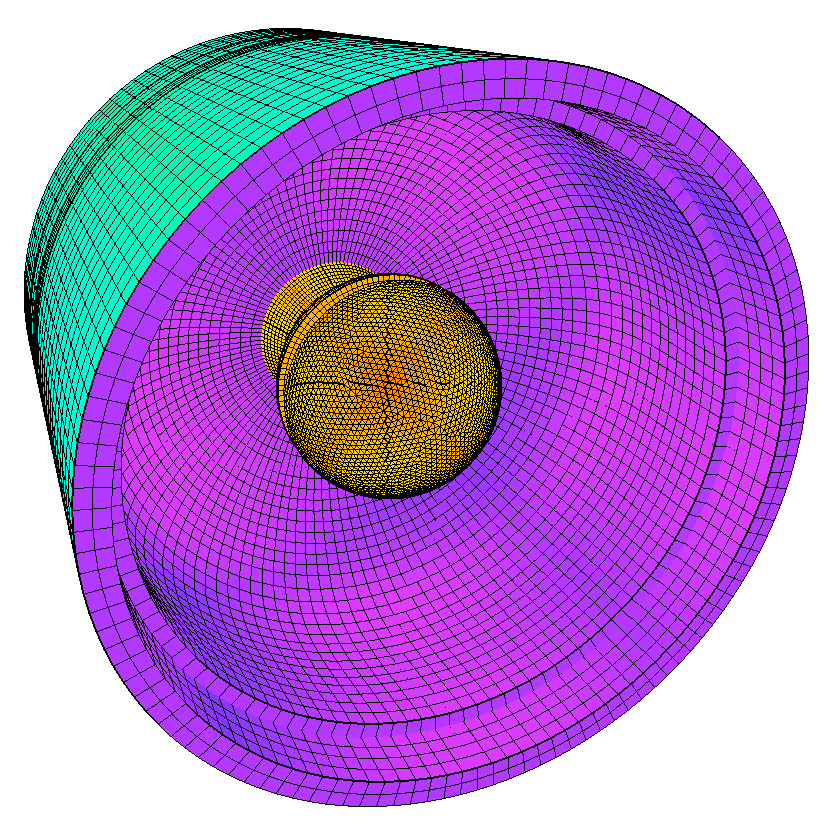
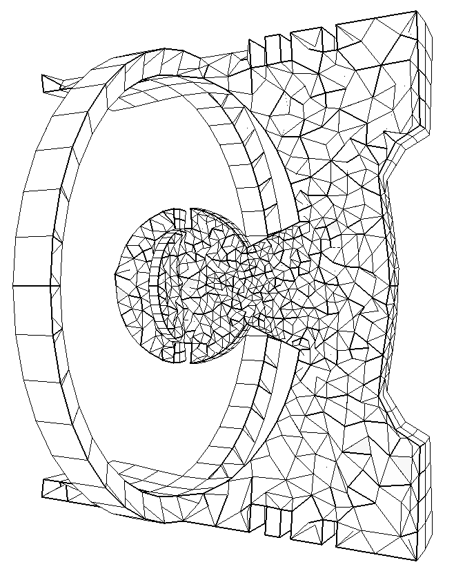
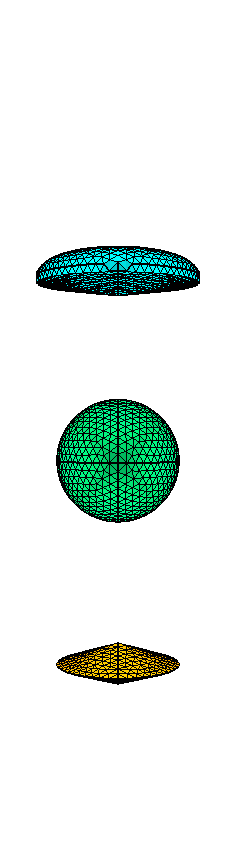
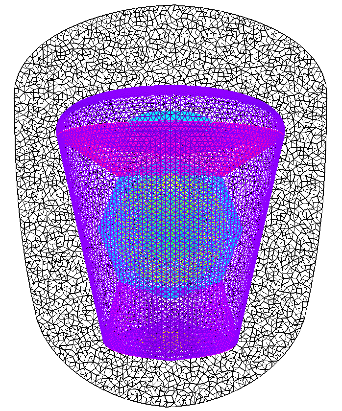
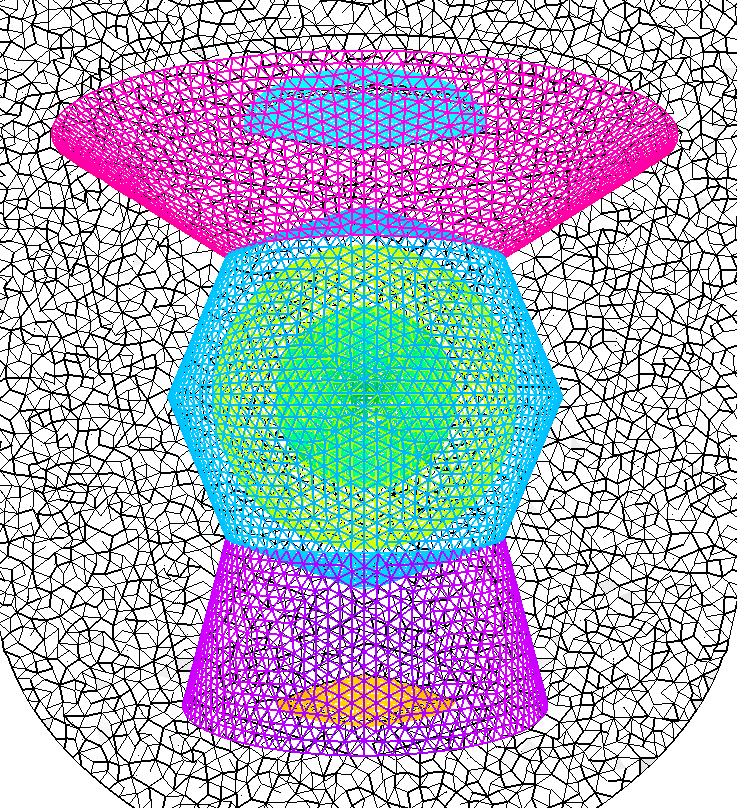
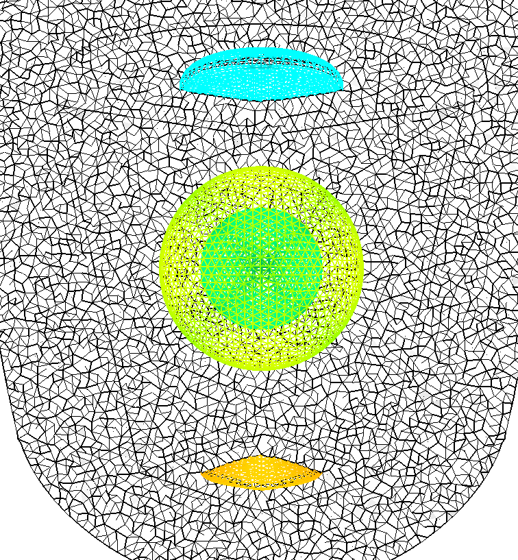
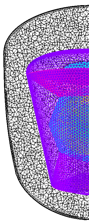
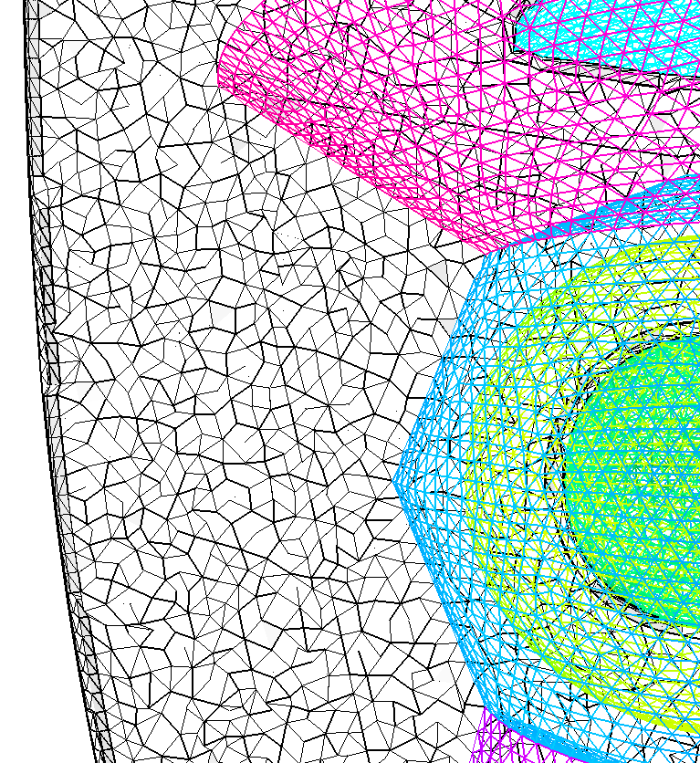
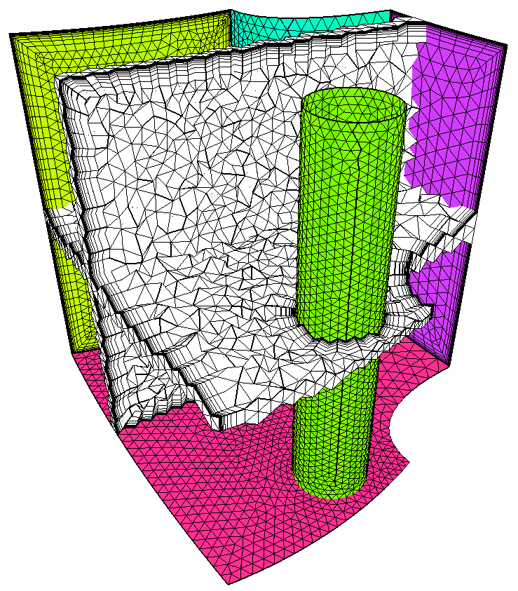
Multi-material assembly with SNS layers.The previous multi-material case
is suitable for an isotropic mesh or one with SNS layers. If the solid objects
in this case had coatings they can be modeled using specified normal spacing
(SNS). Here there is a thin inner and outer coating with two thicker inner
coating layers. An immediate transition to the outer fully isotropic region is
specified with the option -snsr 1. See the documentation for more information
on options related to SNS mode. Appropriate grid boundary conditions are set
within the surface grid file and the mesh can be generated with the following.
Note that in this case an all tetrahedral mesh will be generated. If prisms are
desired in the SNS region then an -snsc option should be used in place of the
-sns option. Also, none of the embedded/transparent surfaces are set to
generate an attached SNS region. If any of them were that would create separate
volumes (and for AFLR3 that would be separate cases). In addition some of those
surfaces are multiply connected (non-manifold) and that is not at present
allowed for BL or SNS generating embedded/transparent surfaces.
aflr3 -i em -sns -snss 0,0.005,0.02,0.07,0.075 -snsr 1
If the input surface mesh does not contain grid boundary conditions then they
can be completely specified on the command line using option flags as shown
below. See documentation for more information on grid boundary condition
values. Here a Grid_BC value of 1 denotes a standard solid surface, a value of
-1 denotes an SNS generating solid surface, and a value of 5 denotes an
embedded or transparent surface that has volume mesh on both sides. For this
case the inner solid objects are ID=2, ID=8, and ID=14; the transparent objects
are ID=3, ID=4, ID=5, ID=6, and ID=9; and the outer solid object is ID=7.
aflr3 -i em -BC_IDs 2,3,4,5,6,7,8,9,14 -Grid_BC_Flag
-1,5,5,5,-1,-1,5,-1 \
-sns -snss 0,0.005,0.02,0.07,0.075 -snsr 1
Duct with primary inflow, two curved periodic inflow/outflow surfaces, and
an internal offset tube. The inlet and exit surfaces are treated as
periodic surfaces that intersect the BL region and are rebuilt within AFLR3.
This is a slice of a larger configuration that is like a ring formed of
multiple pieces the same as this case and connected at the curved periodic
boundaries. Note that appropriate grid boundary conditions are set within the
surface grid file. Also a PSDATA file is provided to specify the surface IDs
for the periodic pair, the translation vector (from a common point on the
periodic pair), and the rotation matrix. SolidMesh generates this file
or the equivalent data can be specified on the command line. However, for
complex cases that is tedious and some procedure to generate the PSDATA file
data automatically is recommended. The input surface meshes for a periodic pair
must match exactly when translated and rotated. This also means that the
translation vector and rotation matrix data must be specified with full
precision, otherwise the pair will not match exactly. The output mesh will
contain a similarly matching pair with a periodic (exactly the same) rebuilt
surface mesh and BL region (on the surface). Evidence of the internal tube is
reflected on the nearby rebuild surface (one less BL layer is produced and the
BL normals align with the tube) and the opposite periodic surface has the exact
same output surface mesh and features (even though it is farther from the
tube).
aflr3 -i periodic_duct -blds 0.00002 -blc
If appropriate grid boundary conditions are not set in the input surface mesh
file then option flags can be used to specify appropriate values. See
documentation for more information on grid boundary condition values. Also
command line arguments can be used to set the surface IDs for a periodic pair,
the translation vector, and the rotation matrix. See documentation for more information.
For this case the inner sphere is ID=1, the spacing control surface is ID=2,
the spacing control surface is ID=2, the spacing control surface is ID=2, the
spacing control surface is ID=2, and the outer sphere is ID=4. The -no_psdata
option is selected to force AFLR3 to use the command line arguments for the
periodic pair instead of those from the PSDATA file.
aflr3 -i periodic_duct -blds 0.00002 -blc -no_psdata \
-BC_IDs 1,2,3,4,5,6,10,11,12 -Grid_BC_Flag -1,-1,2,-1,2,2,-1,-1,-1 \
-npsurf 1 -PS_IDs 6,5 -PS_XPS0s 0,10,0 \
-PS_TMs 0.984807753012,0.173648177667,0.0,\
-0.173648177667,0.984807753011,-1.45784439342e-06,\
-2.53152022229e-07,1.43569646133e-06,1.0
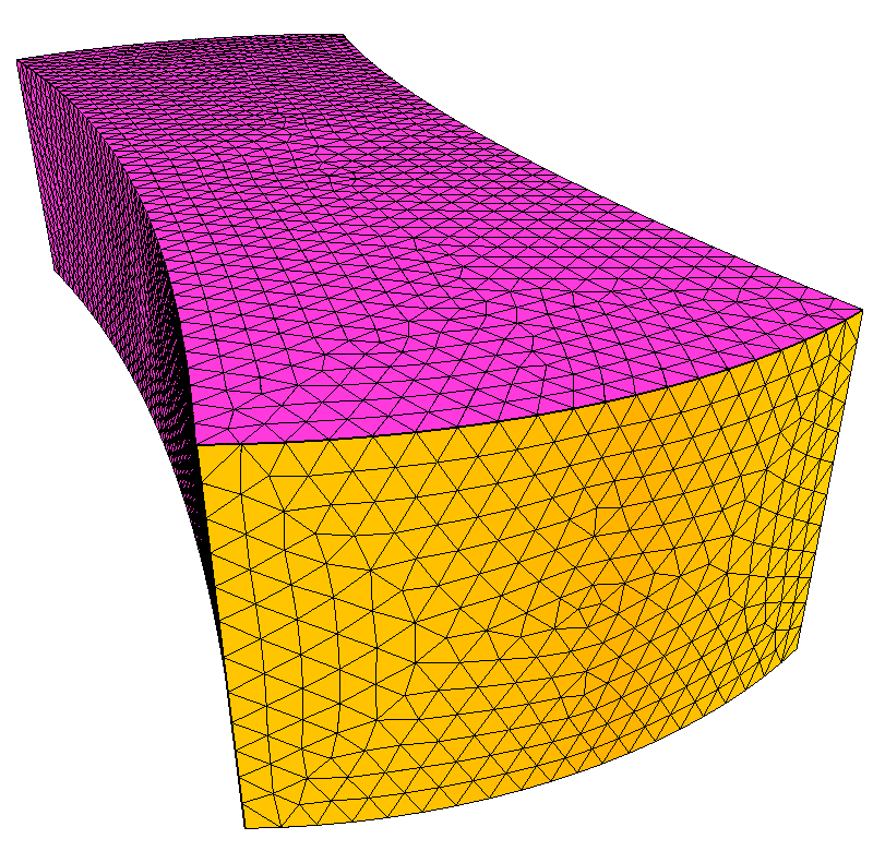
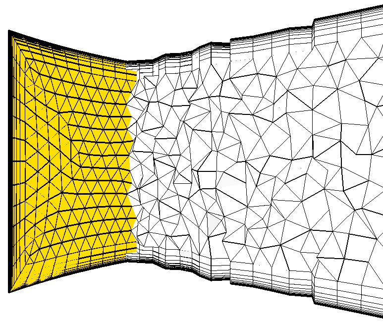
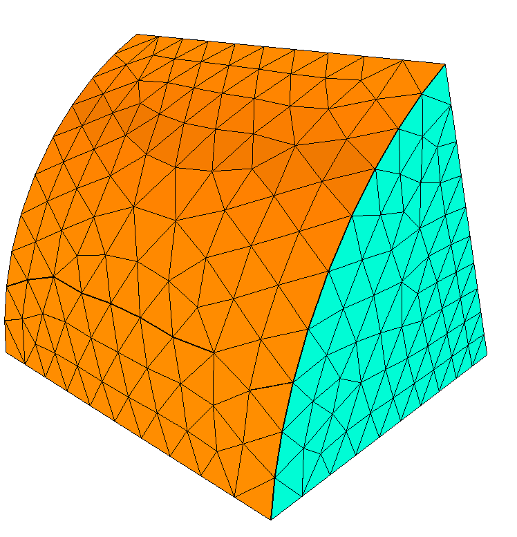
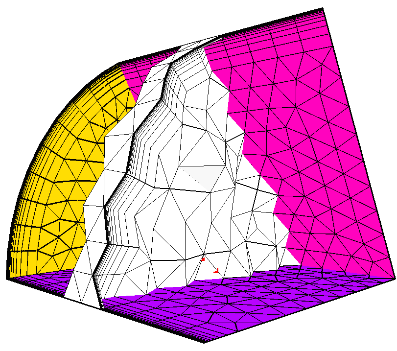
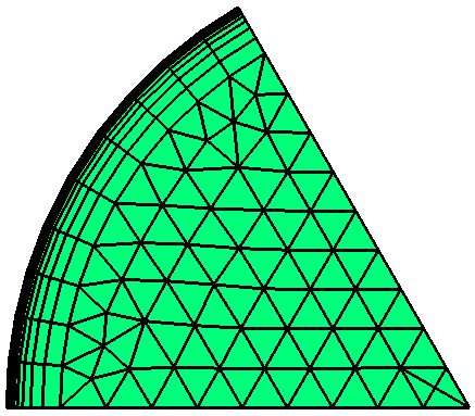
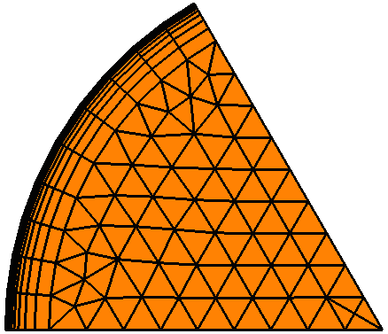
60˚
wedge with periodic symmetry planes and periodic top and bottom surfaces. The
periodic surfaces are treated as surfaces that intersect the BL region and are
rebuilt within AFLR3. Note that appropriate grid boundary conditions are
set within the surface grid file. Also a PSDATA file is provided to specify the
surface IDs for the periodic pairs, the translation vectors (from a common
point on the periodic pairs), and the rotation matrices. SolidMesh
generates this file or the equivalent data can be specified on the command line.
The input surface meshes for each periodic pair must match exactly when
translated and rotated. This also means that the translation vector and
rotation matrix data must be specified with full precision, otherwise the pair
will not match exactly. The output mesh will contain similarly matching pairs
with a periodic (exactly the same) rebuilt surface mesh and BL region (on each
surface).
aflr3 -i wedge60 -blds 0.00002 -blc
If appropriate grid boundary conditions are not set in the input surface mesh
file then option flags can be used to specify appropriate values. See
documentation for more information on grid boundary condition values. Option
flags can be added to set the grid boundary condition flag for all surfaces.
Also command line arguments can be used to set the surface IDs for periodic
pairs, the translation vectors, and the rotation matrices. See documentation
for more information. For this case the front and back periodic surfaces are
ID=1 and ID=2; the periodic symmetry surfaces are ID=3 and ID=4; and the outer
wall is ID=7. The -no_psdata option is selected to force AFLR3 to use the
command line arguments for the periodic pair instead of those from the PSDATA
file.
aflr3 -i wedge60 -blds 0.00002 -blc -no_psdata \
-BC_IDs 1,2,3,4,7 -Grid_BC_Flag 2,2,2,2,-1 \
-npsurf 2 -PS_IDs 1,2,3,4 -PS_XPS0s 0,0,-10,5,8.66025403784,0 \
-PS_TMs 1,0,0,0,1,0,0,0,1,0.5,0.866025403784,0,-0.866025403784,0.5,0,0,0,1
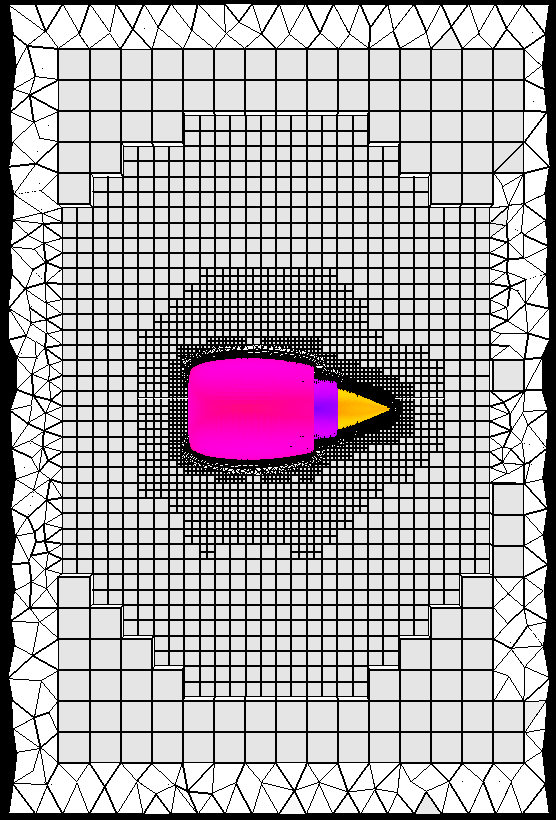
Missile
with nozzle, plume and near-field control surface with a Cartesian interior
core (ICE) mesh. This configuration is similar to the previous missile case,
except that a fully unstructured triangular face surface mesh is used. The
near-field control surface is modeled as an embedded/transparent source
surface. A transparent source surface is used here to control spacing nearby
the missile. The source surface provides a means of determining the appropriate
local length scale. Outside of the source surface the element size increases
relatively rapidly with growth out to the very coarse far-field. Note that with
an embedded/transparent source surface only the surface points are inserted
into the volume mesh. If any of those points do not lie in the volume mesh
region they are ignored. The plume in this configuration is also modeled as an
embedded/transparent source surface to provide a slight increase in mesh
resolution within the plume region.A nozzle inlet is included that is treated
as a surface that intersects the BL region and is rebuilt within AFLR3.
Note that appropriate grid boundary conditions are set within the surface grid
file. The option -ice is added to generate a Cartesian interior core
mesh of hexahedral elements with varying element size. Note that the
current implementation of the Cartesian interior core mode is not compatible
with an embedded/transparent surface that generates a BL region. This
restriction will be eliminated in the future.
aflr3 -ice -i missile_ic -o missile_ic_bl.b8.ugrid -blc
-blds 0.0001
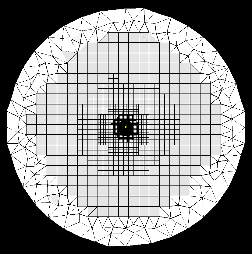
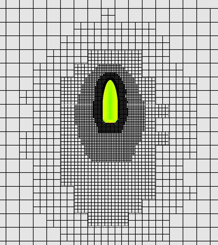
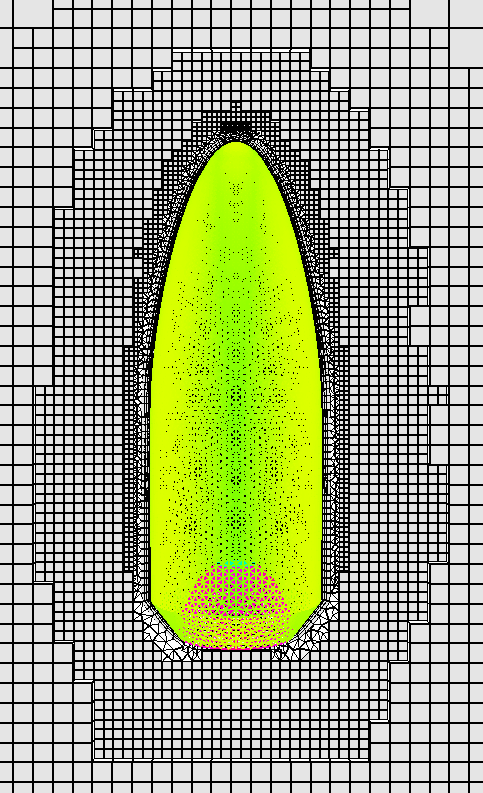
In the above case the element size distribution in the field is similar to that
generated without the -ice option (unstructured tetrahedral core mesh).
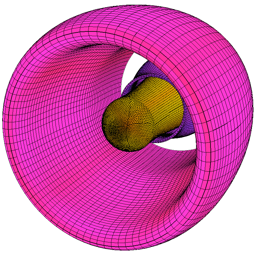
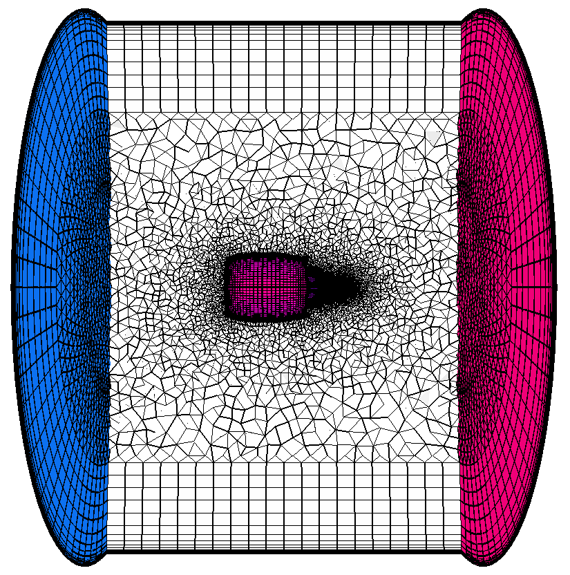
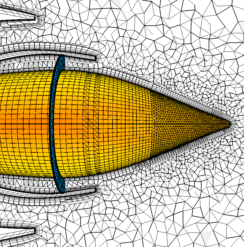
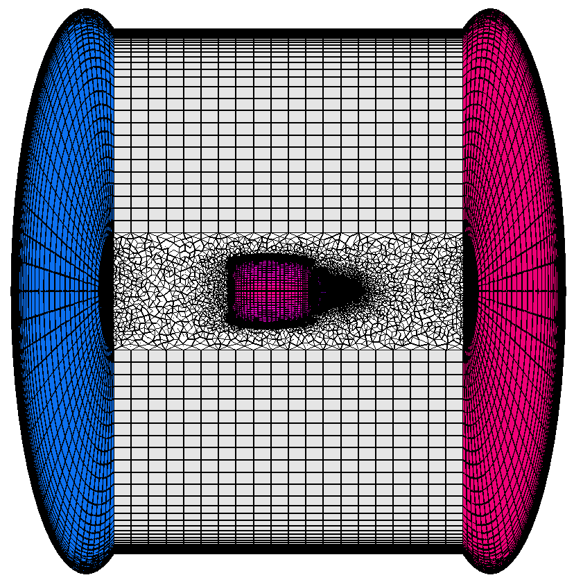
Aircraft nacelle with engine inside a section of wind tunnel with a Cartesian
interior core (ICE) mesh. This configuration is similar to
the previous nacelle case, except that surfaces for the compressor fan and
turbine blades are not included and a BL is not generated on the tunnel walls
(primarily to allow that region to be filled with a Cartesian interior core
mesh).Note that appropriate grid boundary conditions are set within the surface
grid file. Much of the surface mesh contains quad faces. The option -ice is
added to generate a Cartesian interior core mesh of hexahedral elements with
varying element size. Note that the current implementation of the Cartesian
interior core mode will not allow hexahedral elements to be generated in the BL
region. This restriction will be eliminated in the future.
aflr3 -ice -i nacelle_engine_ic -o
nacelle_engine_ic_bl.b8.ugrid -blc -blds 0.0002 -blrm 1.2
In the above case the element size distribution in the field is similar to that
generated without the -ice option (unstructured tetrahedral core mesh).
Nozzle
with constrained/fixed inlet and outlet. In this case it is
assumed that the inlet and outlet surfaces are constrained or fixed and may not
be modified in any way. They are also treated as fixed surfaces that intersect
the BL region. The BL region must match exactly that provided on inlet and
outlet surfaces. This can be the case if one must match up a sub-domain to one
that is meshed by another procedure. It is also relevant to cases that one
wants to mesh as separate domains. An example might be one sub-component of a
large more complex configuration. That would allow remeshing only the
sub-component, if design variations are being studied, instead of remeshing the
entire configuration. Note that AFLR3 BL related parameters should be
used that are as close as possible to those of the other procedure. If that is
not possible then there will be volume mesh distortion near the fixed surface.
Also, it is assumed that the fixed surface was generated using a procedure that
produces a pseudo-structured BL region. The process used here is not
appropriate for matching an arbitrary anisotropic surface mesh. The fixed
surfaces will not be modified, except possibly those with quad faces. If split
face transition from hex elements is allowed then quad faces may be split on
the the fixed surface that could not be matched to the volume BL region. If
pyramid transition is used then quad faces on fixed surfaces will always be
retained. In this case the surface grid on the nozzle wall is made up entirely
of quad faces. Hex elements can be generated in the BL region to reduce overall
element count. The -blc3 option is added to generate hex elements with pyramid
element transition. Use of the -blc2 option instead would generate hex elements
with split face transition to the tetrahedral isotropic mesh region. The
maximum growth rate in the BL region is limited to 1.2. This results in
additional BL region resolution with a typically greater extent. While
appropriate grid boundary conditions may be set within the surface grid file,
they can also be set on the command line (as is often the case with fixed
surfaces). Here appropriate grid boundary conditions are set for the fixed
inlet and outlet along with the BL generating nozzle wall. Note that option
flags that require a list of items must be terminated with a comma if there is
only one item in the list (as is the case here for setting the BL grid boundary
condition on the nozzle wall).
aflr3 -i nozzle_fixed -blc3 -blds 0.0001 -blrm 1.2 -fints
1,2 -bls 3,

Constrained/fixed extracted sub-mesh. The use of a constrained or fixed
surface is useful in cases where one wants to remesh only a small region of an
existing mesh and have only that region vary. Some other procedure is required
to extract the region and would be dependent on the specifics of the cases to
be considered.An example might be comparing variations of one sub-component of
a larger more complex configuration. Two example cases that have been extracted
from a volume mesh are provided here. Each case includes a solid BL generation
surface surrounded by a constrained surface that intersects the BL region (the
grid boundary condition is set to a fixed surface that intersects the BL
region). Both cases are run with the same BL parameter options as the larger
volume mesh was. The first case should be run with the following options.
aflr3 -i submesh1 -blc3 -refx 100 -y+ 1 -bldel 3 -bls 1,2
-fints 3,
The second case should be run with the following options.
aflr3 -i submesh2 -blc3 -blds 0.001 -bldel 0.15 -bls 1,
-fints 2,
Simple sphere BL with metric blending. The use of metric blending is
useful in cases where the BL region may terminate with high-aspect ratio
elements. In these cases the transition to isotropic elements can be very
abrupt. With metric blending the transition is more gradual. In this case we
artificially end the BL region after 24 layers. Without metric blending this
case can be run with the following options.
aflr3 -blc -blds 0.001 -blrm 1.2 nbl=24
To add metric blending this case should be run with the following options. Note
that in this case, metric blending is selected with growth and the parameter
cdfrsrc controls the metric growth rate.
aflr3 -i spheres_1_3_sym -blc -blds 0.001 -blrm 1.2
nbl=24 mmetblbl=2 cdfrsrc=1.05
Metric
blending may also be used with surfaces that intersect the BL region, as in the
following case with a symmetry plane (same as previous with domain cut in
half). The symmetry plane is regenerated with appropriate metric blending to
match the volume mesh. The same options as the previous case are used.
aflr3 -i spheres_1_3_sym -blc -blds 0.001 -blrm 1.2
nbl=24 mmetblbl=2 cdfrsrc=1.05
Constrained/fixed extracted sub-mesh. The use of a constrained or fixed
surface is useful in cases where one wants to remesh only a small region of an
existing mesh and have only that region vary. Some other procedure is required
to extract the region and would be dependent on the specifics of the cases to
be considered.An example might be comparing variations of one sub-component of
a larger more complex configuration. Two example cases that have been extracted
from a volume mesh are provided here. Each case includes a solid BL generation
surface surrounded by a constrained surface that intersects the BL region (the
grid boundary condition is set to a fixed surface that intersects the BL
region). Both cases are run with the same BL parameter options as the larger
volume mesh was. The first case should be run with the following options.
aflr3 -i submesh1 -blc3 -refx 100 -y+ 1 -bldel 3 -bls 1,2
-fints 3,
The second case should be run with the following options.
aflr3 -i submesh2 -blc3 -blds 0.001 -bldel 0.15 -bls 1,
-fints 2,
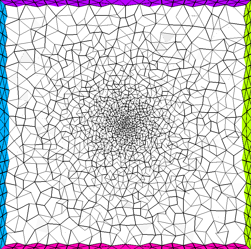
Mesh Sizing
In
default mode AFLR3 determines element sizing based on interpolation
between boundary points (and source points, if any). As mesh generation
advances the sizing is propagated by continued interpolation locally.
Alternatively, an external sizing function can be coded and linked with the
executable. A built-in external sizing function is provided for testing and
example. By itself it is not useful for practical problems. However, developers
can integrate specialized sizing functions within the AFLR3 executable.
The built-in function simply creates a continuous field that varies radially
from the center of the domain outward to the boundaries. At the center the
sizing is smaller than specified at the boundaries. Another alternative for
sizing is to use a background mesh and function file for interpolation. If the
files case_name.back.b8.ugrid and case_name.back.sfunc exist then it is assumed
that use of a background mesh is desired. Note that any supported and readable
volume mesh and function file format and type are equally as acceptable as
.b8.ugrid and .sfunc. The case name case_name must be the same as the input
surface mesh file. The option flag -no_back can be added to ignore these files.
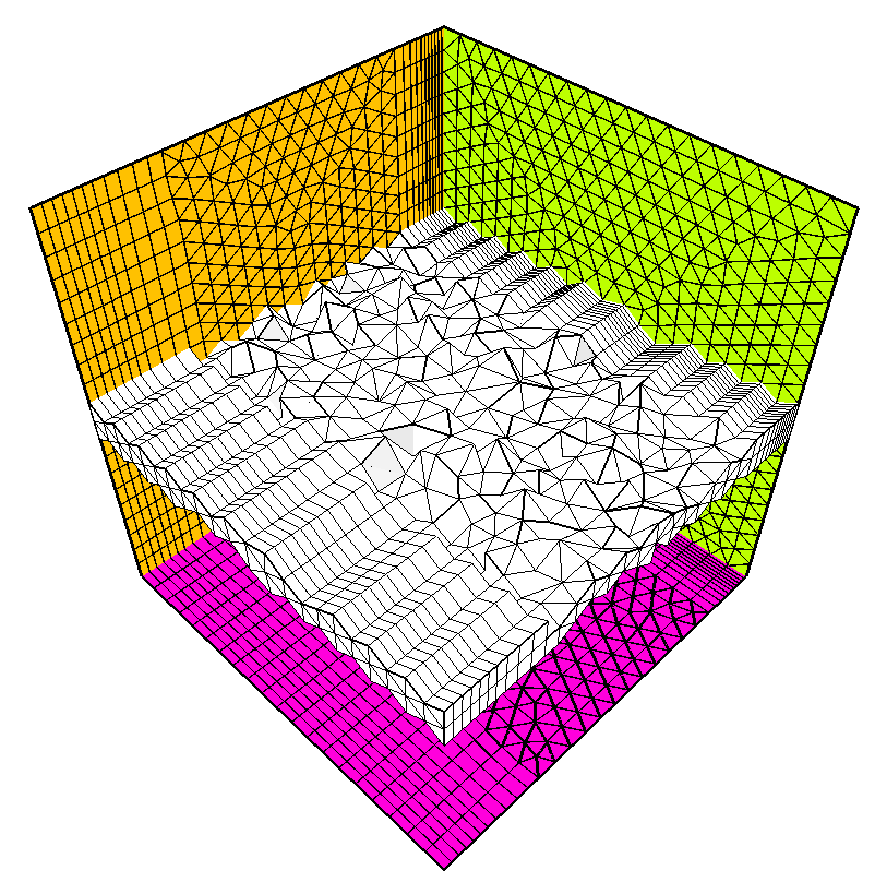
Cube
with external isotropic sizing function. The following example uses
the built-in external sizing function. If an alternative routine is created
then use of that function is controlled in the same manner. This
case also creates a background grid sizing field that will be used in the next
case. The option flag -ext activates use of the external sizing function and
the flag mwbgfunc=1 (not required for normal usage) simply creates an output
function file box.back.sfunc which contains the isotropic sizing for each mesh
vertex.
aflr3 -i cube -ext mwbgfunc=1
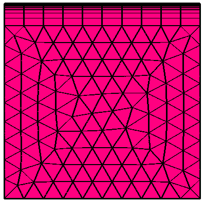
Cube
with background mesh for interpolation of isotropic sizing.
In this test case the background mesh sizing field is derived from the previous
case. It could also be generated from another code that bases the sizing on the
computed physics or other criteria. The resulting mesh is equivalent to the
previous case (on which it is based). However, it does differ since here we are
interpolating rather than determining the sizing analytically. No option flags
are required to activate the background mesh option. If the files exist and the
flag -no_back is not used then the option is automatically selected.
cp box.b8.ugrid box.back.b8.ugrid
aflr3 -i cube
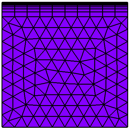
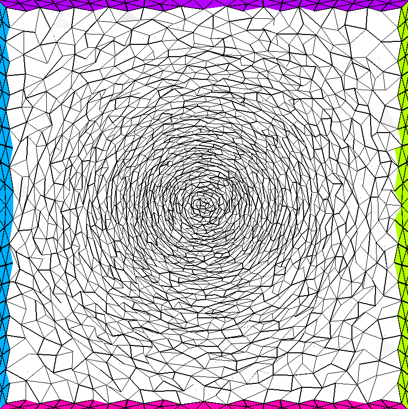
Cube with external anisotropic metric based sizing function. When metric
space tensors are used (mmet=1) the built-in function simply creates a
continuous field that varies in anisotropy and size radially from the center of
the domain outward to the boundaries. At the center the aspect ratio is larger
(elements are more flat) and the maximum element size is somewhat smaller. The
following example uses the built-in external sizing function with metric based
anisotropy. In this case the background mesh function file will contain both
isotropic sizing and the metric directional sizing fields.
aflr3 -i cube -ext mmet=1 mwbgfunc=1
Cube
with background mesh for interpolation of metric based sizing.
In this test case the background mesh sizing field is derived from the previous
case. It could also be generated from another code that bases the sizing on the
computed physics or other criteria. The resulting mesh is equivalent to the
previous case (on which it is based). However, it does differ since here we are
interpolating rather than determining the sizing analytically. No option flags
are required to activate the background mesh option. If the files exist and the
flag -no_bg is not used then the option is automatically selected. The metric
option mmet=1 must be included to use a metric based directional sizing.
cp box.b8.ugrid box.back.b8.ugrid
aflr3 -i cube mmet=1